
Appearance
PI-ZN010-F1-1 FPGA Tutorial

Alinx Electronic Limited
Company Website: www.en.alinx.com
Service Hotline: +86 21 67676997
Technical Support : technical@alinx.com
Document Information
| Item | Content |
| Document Type | Tutorial |
| Product Model | PI-ZN010-F1-1 |
| Document Version | V1.0 |
| Prepared by | Alinx Electronic Limited |
| Release Date | 2026.11.13 |
Document Revision History
| Version | Date | Section | Revision Summary |
| V1.0 | 2026.11.13 | All | Initial Release |
Creating a Vivado Project with a Batch Script
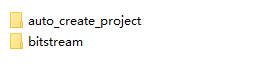
To save users the time spent downloading materials, a batch-based method for creating Vivado projects is provided. Under each folder there are two subfolders: auto_create_project is the batch folder, and bitstream contains the bit files so that the functions can be verified quickly.
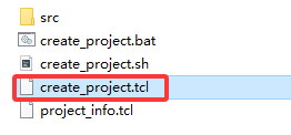
create_project.tcl is the script that creates the Vivado project.
The two commands at the very bottom of this file compile the project and generate the bit file. By default the project is not compiled. You can decide according to your own needs whether to compile the project; if you do, remove the comment marks from these two lines (that is, delete the #). Compilation takes a fairly long time.

Under Windows, enter the auto_create_project folder and edit create_project.bat, replacing the vivado.bat path with the path to Vivado on your own computer, then save the file.
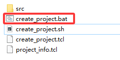

Double-click create_project.bat to start creating the Vivado project, and wait until the batch file finishes running.
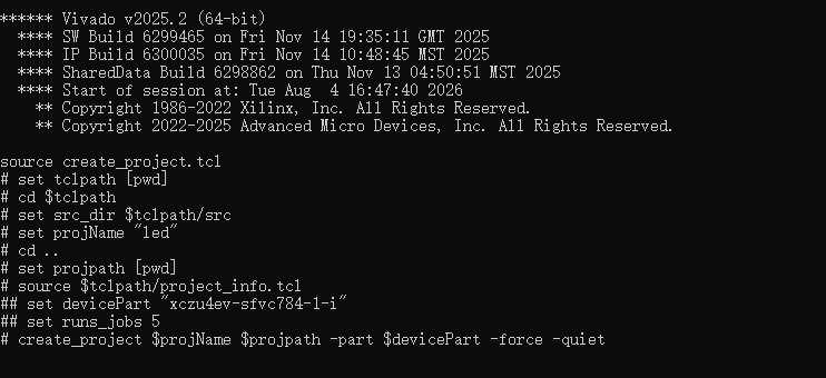
Under Linux, likewise enter the auto_create_project folder and edit create_project.sh, replacing it with the path to Vivado on your own computer, then save the file.
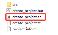

Enter the chmod command to change the file permissions, then run the create_project.sh file.


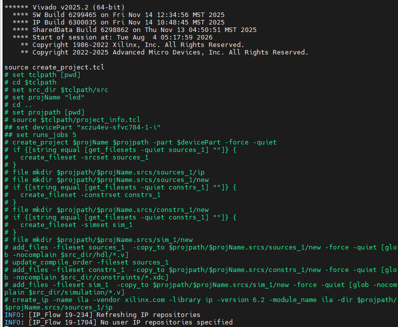
The run process is as follows; simply wait until the batch file finishes running and the project is ready to use.
Chapter 1 Introduction to ZYNQ
The highlight of the Zynq series is that the FPGA contains a complete ARM processing subsystem (PS). Every Zynq processor includes a Cortex-A9 processor, and the whole device is built around this processor. The processing subsystem integrates a memory controller and a large number of peripherals, so that the Cortex-A9 core in Zynq-7000 is completely independent of the programmable logic. That is to say, even if the programmable logic (PL) is not used for the moment, the ARM processing subsystem can still work on its own. This is fundamentally different from earlier FPGAs: the device is centred on the processor.
Zynq is made up of two major functional blocks, the PS part and the PL part — in plain terms, the ARM SoC part and the FPGA part. The PS integrates two ARM Cortex™-A9 processors, the AMBA® interconnect, on-chip memory, external memory interfaces and peripherals. These peripherals mainly include a USB bus interface, an Ethernet interface, SD/SDIO interfaces, an I2C bus interface, a CAN bus interface, a UART interface, GPIO, and so on.
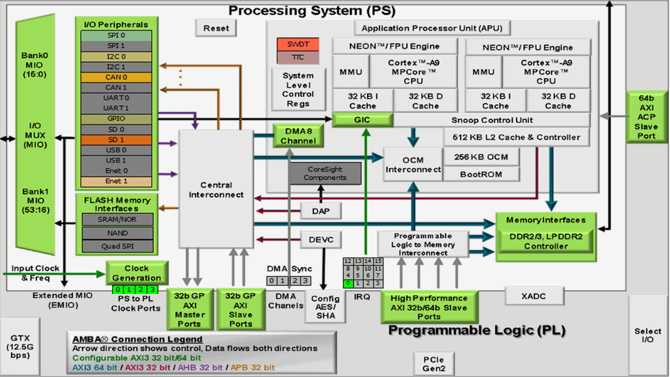
Overall block diagram of the ZYNQ chip
PS: Processing System — the ARM SoC part that is unrelated to the FPGA.
PL: Programmable Logic — the FPGA part.
The PL part is the same as in the 7 series; the corresponding 7 series devices can be found in document DS190.

1.1 PS-PL Interconnect Technology
As the first product to tightly combine a high-performance ARM Cortex-A9 series processor with a high-performance FPGA in a single chip, ZYNQ needs an efficient on-chip interconnect path between the high-performance processor and the FPGA in order to achieve high-speed communication and data exchange between the ARM processor and the FPGA, and to exploit the performance advantages of both. Designing an efficient PL-PS data exchange path is therefore of paramount importance in ZYNQ chip design, and it is one of the keys to the success of a product design. This section mainly introduces the connection between PS and PL, so that users understand the technology of the PS-PL connection.
In fact, in specific designs we usually do not need to do much work on the connection itself. After we add an IP core, the system automatically connects that IP core to the processor using the AXI interface; we only need to make a few additional adjustments.
AXI stands for Advanced eXtensible Interface. It is an interface protocol that Xilinx introduced starting with its 6 series FPGAs, and it mainly describes the way data is transferred between a master device and a slave device. It continues to be used in ZYNQ, at version AXI4, so you will often see AXI4.0 referred to; all internal devices in ZYNQ have AXI interfaces. AXI is in fact part of AMBA (Advanced Microcontroller Bus Architecture), proposed by ARM. It is a high-performance, high-bandwidth, low-latency on-chip bus, and it is also used to replace the earlier AHB and APB buses. The first version of AXI (AXI3) was included in AMBA3.0, released in 2003, and the second version of AXI (AXI4) was included in AMBA 4.0, released in 2010.
The AXI protocol mainly describes the way data is transferred between a master device and a slave device, and the master and the slave establish a connection through handshake signals. When the slave is ready to receive data, it asserts the READY signal. When the master's data is ready, it asserts and holds the VALID signal, indicating that the data is valid. Data transfer starts only when both VALID and READY are asserted. As long as both signals remain asserted, the master continues to transfer the next data item. The master can deassert VALID, or the slave can deassert READY, to terminate the transfer. The AXI protocol is shown in the figure: at T2 the slave's READY signal is asserted, at T3 the master's VALID signal is asserted, and the data transfer begins.
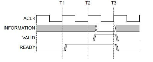
AXI handshake timing diagram
In ZYNQ, three buses are supported: AXI-Lite, AXI4 and AXI-Stream. Table 5-1 shows the characteristics of these three AXI interfaces.
| Interface Protocol | Characteristics | Application |
| AXI4-Lite | Address/single data transfer | Low-speed peripherals or control |
| AXI4 | Address/burst data transfer | Bulk data transfer |
| AXI4-Stream | Data only, burst transfer | Data streams and media streams |
AXI4-Lite:
It is lightweight and simple in structure, and is suitable for small batches of data and simple control applications. It does not support burst transfer; a single read or write can only access one word (32 bits) at a time. It is mainly used to access low-speed peripherals and to control peripherals.
AXI4:
Its interface is similar to AXI-Lite, but with one additional function: burst transfer, which allows a continuous region of addresses to be read or written in one go. In other words, it has the burst function for data reads and writes.
Both of the above use the memory-mapped control method, that is, the ARM maps the user-defined IP core into a certain address space for access, and reading and writing it is like reading and writing your own on-chip RAM. Programming is convenient and development is relatively easy. The cost is higher resource usage, since additional signal lines are required: read address, write address, read data, write data and write response lines.
AXI4-Stream:
This is a continuous streaming interface that does not require address lines (much like a FIFO, where you simply keep reading or keep writing). For this type of IP, the ARM cannot control it through the memory-mapped method described above (a FIFO has no concept of an address at all), so a conversion device is required, for example an AXI-DMA module, to convert the memory-mapped interface into a streaming interface. AXI-Stream is suitable for many applications: video stream processing, communication protocol conversion, digital signal processing, wireless communication, and so on. In essence, all of these build a data path for a stream of values, forming a continuous data stream from a source (such as ARM memory, DMA, a wireless receive front end, etc.) to a sink (such as an HDMI monitor, a high-speed AD audio output, etc.). This interface is suitable for real-time signal processing.
The AXI4 and AXI4-Lite interfaces contain 5 different channels:
Read Address Channel
Write Address Channel
Read Data Channel
Write Data Channel
Write Response Channel
Each of these channels is an independent AXI handshake protocol. The following two figures show the read and write models respectively:
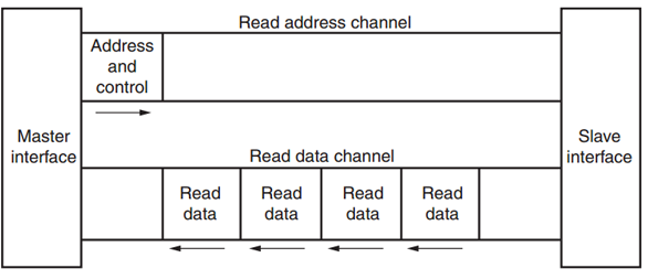
AXI read data channels
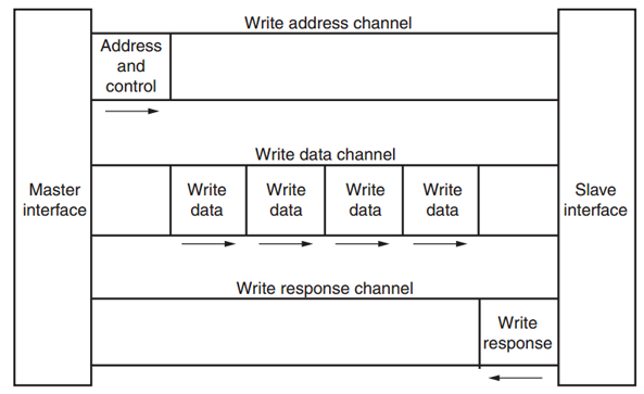
AXI write data channels
The AXI bus protocol is implemented in hardware inside the ZYNQ chip, including 9 physical interfaces: AXI-GP0 to AXI-GP3, AXI-HP0 to AXI-HP3, and the AXI-ACP interface.
The AXI_ACP interface is an interface defined under the ARM multicore architecture; it is known as the Accelerator Coherency Port. It is used to manage AXI peripherals without caches, such as DMA, and on the PS side it is a Slave interface.
The AXI_HP interfaces are high-performance/high-bandwidth interfaces of the AXI3.0 standard. There are four of them in total, and the PL module connects to them as a master device. They are mainly used by the PL to access memory on the PS side (DDR and On-Chip RAM).
The AXI_GP interfaces are general-purpose AXI interfaces. There are four of them in total, including two 32-bit master interfaces and two 32-bit slave interfaces.
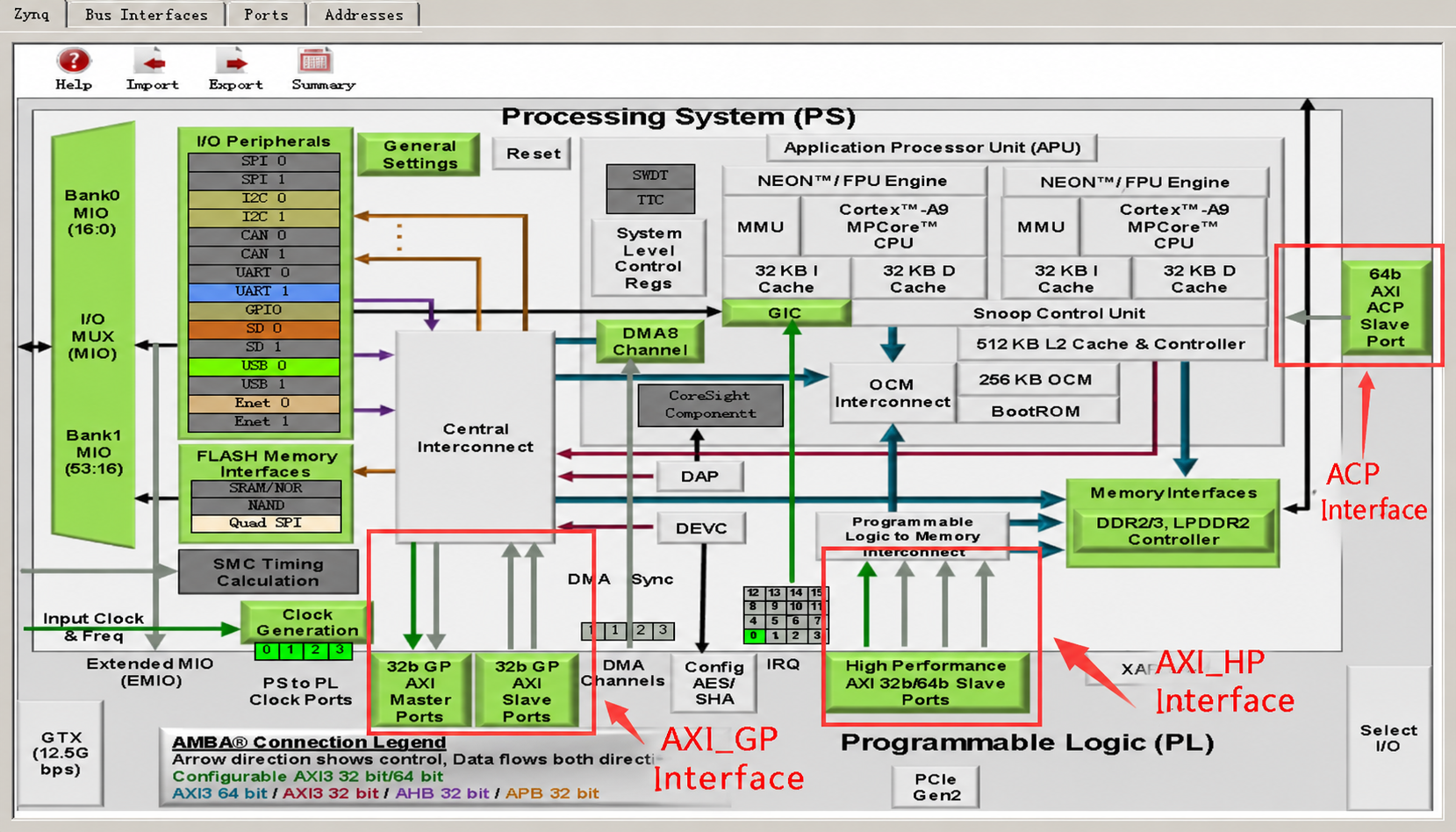
As can be seen, only two of the AXI-GP ports are Master Ports, that is, host interfaces; the remaining 7 ports are Slave Ports. A host interface has the right to initiate reads and writes, and the ARM can actively access the PL logic through the two AXI-GP host interfaces. In effect, the PL is mapped into a certain address, and reading and writing PL registers is like reading and writing your own memory. The remaining slave interfaces are passive interfaces: they accept reads and writes coming from the PL and simply obey them.
In addition, the performance of these 9 AXI interfaces differs. The GP interfaces are 32-bit low-performance interfaces with a theoretical bandwidth of 600MB/s, while the HP and ACP interfaces are 64-bit high-performance interfaces with a theoretical bandwidth of 1200MB/s. Some people may ask: why are the high-performance interfaces not made into host interfaces, so that the ARM could initiate high-speed data transfers? The answer is that the high-performance interfaces do not need the ARM CPU to handle data movement at all; the real mover is the DMA controller located in the PL.
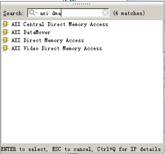
The ARM located on the PS side has direct hardware support for the AXI interface, whereas the PL needs to implement the corresponding AXI protocol using logic. In the Vivado development environment, Xilinx provides ready-made IP such as AXI-DMA, AXI-GPIO, AXI-Dataover and AXI-Stream, all of which implement the corresponding interfaces; you can simply add them from the Vivado IP list to obtain the corresponding functions. The figure below shows the various DMA IP in Vivado:
Below is an introduction to the functions of several commonly used AXI interface IP:
AXI-DMA: implements the conversion from the PS memory to the PL high-speed transmission channel, AXI-HP<---->AXI-Stream.
AXI-FIFO-MM2S: implements the conversion from the PS memory to the PL general-purpose transmission channel, AXI-GP<----->AXI-Stream.
AXI-Datamover: implements the conversion from the PS memory to the PL high-speed transmission channel, AXI-HP<---->AXI-Stream, except that this time it is fully controlled by the PL and the PS is completely passive.
AXI-VDMA: implements the conversion from the PS memory to the PL high-speed transmission channel, AXI-HP<---->AXI-Stream, but it is dedicated to two-dimensional data such as video and images.
AXI-CDMA: this moves data from one location in memory to another, done by the PL, without the CPU being involved.
How to use these IP will be illustrated in later chapters. Sometimes users need to develop their own custom IP to communicate with the PS; in that case the corresponding IP can be generated using the wizard. A user-defined IP core can have AXI4-Lite, AXI4, AXI-Stream, PLB and FSL interfaces. The latter two are not used because the ARM side does not support them.
With the official IP described above and the custom IP generated by the wizard, users actually do not need to understand AXI timing in great detail (unless a problem really occurs), because Xilinx has encapsulated all the details related to AXI timing; users only need to focus on their own logic implementation.
Strictly speaking, the AXI protocol is a point-to-point master-slave interface protocol. When multiple peripherals need to exchange data with each other, an AXI Interconnect module must be added — that is, an AXI interconnect matrix. Its function is to provide a switching mechanism that connects one or more AXI master devices to one or more AXI slave devices (somewhat similar to the switching matrix inside a network switch).
This AXI Interconnect IP core can support up to 16 master devices and 16 slave devices. If more interfaces are needed, several more IP cores can be added.
The basic connection modes of AXI Interconnect are as follows:
N-to-1 Interconnect
to-N Interconnect
N-to-M Interconnect (Crossbar Mode)
N-to-M Interconnect (Shared Access Mode)
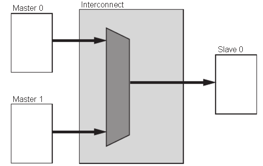
The many-to-one case
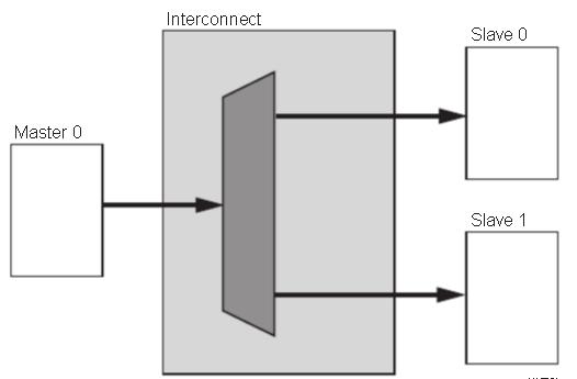
The one-to-many case
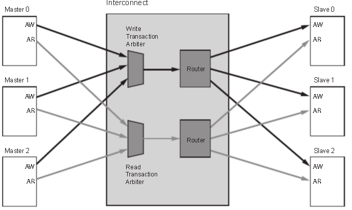
Many-to-many read and write address channels
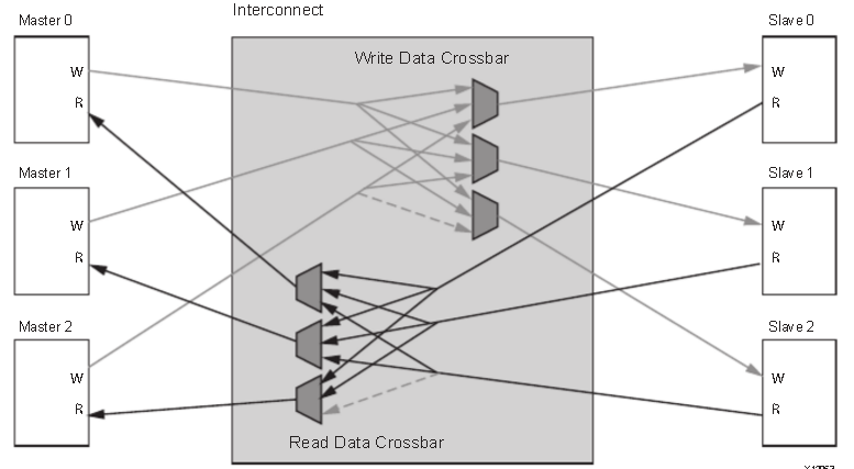
Many-to-many read and write data channels
The AXI interface devices inside ZYNQ are interconnected in exactly this interconnect-matrix way, which guarantees both the efficiency of data transfer and the flexibility of connection. In Vivado, Xilinx provides us with an IP core that implements this interconnect matrix, axi_interconnect; we only need to instantiate it.
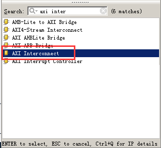
AXI Interconnect IP
1.2 Introduction to the ZYNQ Chip Development Flow
Because ZYNQ integrates a CPU and an FPGA together, developers need to design both the ARM operating system applications and device drivers, and the hardware logic design of the FPGA part. During development it is necessary to understand the Linux operating system and the system architecture, and also to build a hardware design platform between the FPGA and the ARM system. ZYNQ development therefore requires software engineers and hardware engineers to work together on the design and development. This is what is called "software-hardware co-design" in ZYNQ development.
The design and development of the hardware and software systems of a ZYNQ system require the following development environment and debugging tools: Xilinx Vivado.
The Vivado Design Suite implements the design and development of the FPGA part, pin and timing constraints, compilation and simulation, and the RTL-to-bitstream design flow. Vivado is not a simple upgrade of the ISE Design Suite but a completely new design suite. It replaces all the important tools of the ISE Design Suite, such as Project Navigator, Xilinx Synthesis Technology, Implementation, CORE Generator, Constraint, Simulator, Chipscope Analyzer, FPGA Editor and other design tools.
Xilinx SDK (Software Development Kit). SDK is Xilinx's software development kit. On the basis of the Vivado hardware system, the system automatically configures a number of important parameters, including tool and library paths, compiler options, JTAG and flash settings, debugger connections and the bare-metal board support package (BSP). SDK also provides drivers for all supported Xilinx IP hard cores. SDK supports the co-debugging of IP hard cores (on the FPGA) and processor software; we can use high-level C or C++ to develop and debug ARM and FPGA systems and test whether the hardware system works properly. The SDK software is also bundled with Vivado and does not need to be installed separately.
ZYNQ development also follows the hardware-first, software-second approach. The specific flow is as follows:
1. Create a new project in Vivado and add an embedded source file.
2. In Vivado, add and configure the basic peripherals of the PS and PL parts, or add the custom peripherals that are needed.
3. In Vivado, generate the top-level HDL file and add the constraint file. Then compile and generate the bitstream file (*.bit).
4. Export the hardware information to the SDK software development environment. In the SDK environment you can write some debugging software to verify the hardware and software, and debug the ZYNQ system separately together with the bitstream file.
5. Generate the FSBL file in SDK.
6. Generate u-boot.elf and the bootloader image in a VMware virtual machine.
7. In SDK, use the FSBL file, the bitstream file system.bit and the u-boot.elf file to generate a BOOT.bin file.
8. In VMware, generate the Ubuntu kernel image Zimage and the Ubuntu root file system. In addition, drivers need to be written for the custom FPGA IP.
9. Put the BOOT, kernel, device tree and root file system files onto the SD card, power on the development board, and the Linux operating system will boot from the SD card.
The above is the typical ZYNQ development flow. However, ZYNQ can also be used as an ARM alone, in which case there is no need to care about the PL-side resources, and it is not much different from traditional ARM development. ZYNQ can also use only the PL part, but the configuration of the PL still has to be done by the PS; that is, it is impossible to burn firmware for the PL alone in the traditional way of programming the flash.
1.3 Skills Required to Learn ZYNQ
Learning ZYNQ places higher demands than learning traditional tools such as FPGA, MCU and ARM development, and mastering ZYNQ is not something that can be achieved overnight.
1.3.1 Software Developers
Computer organization principles
C and C++ languages
Computer operating systems
Tcl scripts
A good foundation in English reading
1.3.2 Logic Developers
Computer organization principles
C language
Fundamentals of digital circuits
Verilog and VHDL languages
A good foundation in English reading
Chapter 2 Introduction to Basic Verilog Modules
2.1 Introduction
This document mainly introduces the basic Verilog modules. A solid foundation is of great help for studying FPGA design in depth.
2.2 Data Types
2.2.1 Constants
Integers: An integer can be expressed in binary (b or B), octal (o or O), decimal (d or D) or hexadecimal (h or H). For example, 8’b00001111 denotes an 8-bit binary integer, and 4’ha denotes a 4-bit hexadecimal integer.
X and Z: X represents an unknown value and z represents a high-impedance value. For example, in 5’b00x11 the third bit is unknown, and 3’b00z indicates that the lowest bit is high impedance.
Underscore: When a number is long, an underscore can be used to separate the digits and improve readability, for example 8’b0000_1111.
parameter: A parameter can be used to define a constant with an identifier; afterwards only the identifier is used, which improves readability and maintainability. For example, defining parameter width = 8; and then reg [width-1:0] a; defines a register 8 bits wide.
Parameter passing: If parameters are defined in one module, they can be passed and modified when another module instantiates that module, as shown below, using #() after the module name.
For example, a module is defined as follows and instantiated as follows.
1
module rom
#(
parameter depth =15,
parameter width = 8
)
(
input [depth-1:0] addr ,
input [width-1:0] data ,
output result
) ;
endmodule


module top() ;
wire [31:0] addr ;
wire [15:0] data ;
wire result ;
rom
#(
.depth(32),
.width(16)
)
r1
(
.addr(addr) ,
.data(data) ,
.result(result)
) ;
endmodule
A parameter can be used to pass parameters between modules, whereas localparam is used only inside this module and cannot be used for parameter passing. localparam is mostly used to define the states of a state machine.
2.3 Variables
A variable is a quantity whose value can change while the program runs. The following mainly introduces several commonly used variable types.
2.3.1 Wire Type
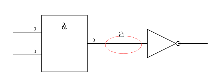
A Wire type variable, also called a net type variable, is used for the physical connection between structural entities, such as between gates. It cannot store a value and is assigned with a continuous assignment statement (assign). It is defined as wire [n-1:0] a;, where n represents the bit width. For example, wire a; assign a = b; connects the node of b to the wire a. As shown in the figure below, the wire between two entities is a Wire type variable.
2.3.2 Reg Type
A Reg type variable, also called a register variable, can be used to store a value and must be used in an always statement. It is defined as
reg [n-1:0] a;, which represents a register n bits wide; for example reg [7:0] a; defines register a 8 bits wide. As shown below, a register q is defined, and the resulting circuit is sequential logic; the figure on the right shows its structure, a D flip-flop.
1
module top(d, clk, q) ;
input d ;
input clk ;
output reg q ;

always @(posedge clk)
begin
    q <= d ;
end

endmodule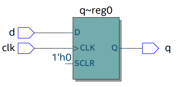
It can also produce combinational logic, such as a data multiplexer. In that case the sensitivity list contains no clock, a reg Mux is defined, and the resulting circuit is combinational logic.
1
module top(a, b, c, d, sel, Mux) ;
input a ;
input b ;
input c ;
input d ;
input [1:0] sel ;
output reg Mux ;

always @(sel or a or b or c or d)
begin
case(sel)
    2'b00 : Mux = a ;
    2'b01 : Mux = b ;
    2'b10 : Mux = c ;
    2'b11 : Mux = d ;
endcase
end

endmodule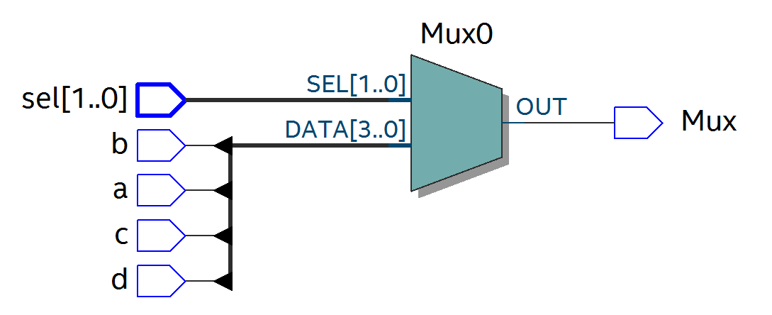
2.3.3 Memory Type
The memory type can be used to define memories such as RAM and ROM. Its form is reg [n-1:0] memory_name[m-1:0], meaning m registers each n bits wide. For example, reg [7:0] ram [255:0] defines 256 8-bit registers, where 256 is the depth of the memory and 8 is the data width.
2.4 Operators
Operators can be divided into the following categories:
1. Arithmetic operators (+, -, *, /, %)
2. Assignment operators (=, <=)
3. Relational operators (>, <, >=, <=, ==, !=)
4. Logical operators (&&, ||, !)
5. Conditional operator (?😃
6. Bitwise operators (~, |, ^, &, ^~)
7. Shift operators (<<, >>)
8. Concatenation operator ({ })
2.4.1 Arithmetic Operators
“+” (addition), “-” (subtraction), “*” (multiplication), “/” (division, for example 7/3 = 2), “%” (modulus, that is, taking the remainder, for example 7%3 = 1, where the remainder is 1).
2.4.2 Assignment Operators
“=” is the blocking assignment and “<=” is the non-blocking assignment. With a blocking assignment, the next assignment statement is executed only after the current one has been executed; it can be understood as sequential execution, and the assignment takes effect immediately. A non-blocking assignment can be understood as parallel execution, where order does not matter; the assignment is performed only after the whole always block has finished executing. The following is an example of blocking assignment:
The code is as follows: The testbench is as follows:
1
module top(din,a,b,c,clk);
input din;
input clk;
output reg a,b,c;
always @(posedge clk)
begin
    a = din;
    b = a;
    c = b;
end
endmodule

`timescale 1 ns/1 ns
module top_tb() ;
reg din ;
reg clk ;
wire a,b,c ;

initial
begin
    din = 0 ;
    clk = 0 ;
    forever
    begin
        #({$random}%100)
        din = ~din ;
    end
end

always #10 clk = ~clk ;

top t0(.din(din),.a(a),.b(b),.c(c),.clk(clk)) ;

endmodule
From the simulation results you can see that on the rising edge of clk the value of a equals din and is immediately assigned to b, and the value of b is assigned to c.

If the assignments are changed to non-blocking, the simulation results are as follows: on the rising edge of clk the value of a is not immediately assigned to b, so b keeps the previous value of a; likewise c keeps the previous value of b.

The clear difference between the two can be seen from their RTL diagrams:
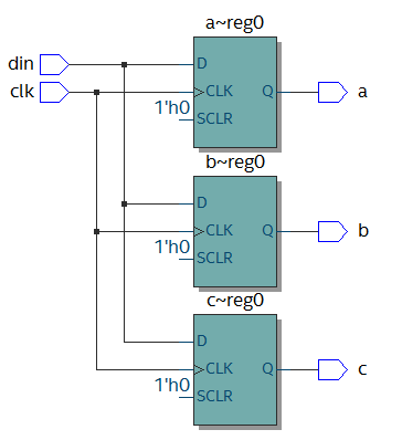
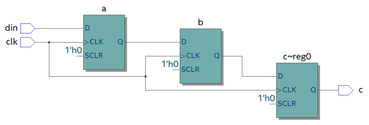
RTL diagram of blocking assignment & RTL diagram of non-blocking assignment
As a general rule, use non-blocking assignment in sequential logic circuits, which avoids race and hazard phenomena during simulation; use blocking assignment in combinational logic, where the value changes immediately after the assignment statement is executed; and blocking assignment must be used in assign statements.
2.4.3 Relational Operators
They express the relationship between two operands, such as a>b or a<b, and are mostly used for conditional tests, for example:
If (a>=b) q <=1’b1 ; else q <= 1’b0 ; meaning that if the value of a is greater than or equal to b, then q is 1, otherwise q is 0.
2.4.4 Logical Operators
“&&” (logical AND of two operands), “||” (logical OR of two operands), “!” (logical NOT of a single operand), for example:
If (a>b && c <d) means the condition is that a>b and c<d; if (!a) means the condition is that the value of a is not 1, that is, 0.
2.4.5 Conditional Operator
“?:” is a conditional test, similar to if else. For example, assign a = (i>8)?1’b1:1’b0 ; tests whether the value of i is greater than 8: if it is greater than 8 then a is 1, otherwise it is 0.
2.4.6 Bitwise Operators
“~” is bitwise inversion, “|” is bitwise OR, “^” is bitwise XOR, “&” is bitwise AND, and “^~” is bitwise XNOR. Except for “~”, which needs only one operand, the others all need two operands, such as a&b and a|b. Their specific application is explained in the combinational logic section later.
2.4.7 Shift Operators
“<<” is the left shift operator and “>>” is the right shift operator. For example, a<<1 means shifting left by 1 bit, and a>>2 means shifting right by two bits.
2.4.8 Concatenation Operator
“{ }” is the concatenation operator, which concatenates several signals bit by bit. For example, {a[3:0], b[1:0]} concatenates the lower 4 bits of a and the lower 2 bits of b into 6 bits of data. In addition, {n{a[3:0]}} means concatenating n copies of a[3:0], and {n{1’b0}} means concatenating n zeros. For example, {8{1’b0}} is expressed as 8’b0000_0000.
2.4.9 Precedence
The precedence of the various operators is as follows:
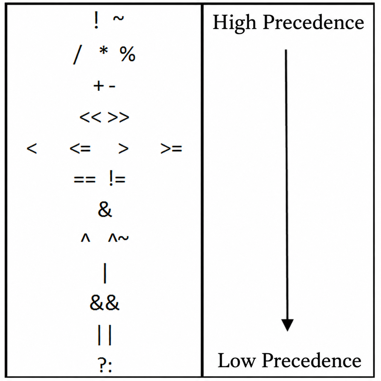
2.5 Combinational Logic
This section mainly introduces combinational logic. The characteristic of a combinational logic circuit is that its output at any moment depends only on the input signals: when the input signals change, the output changes immediately, without depending on the clock.
2.5.1 AND Gate
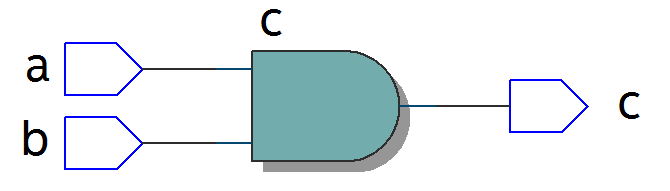
In Verilog, “&” denotes bitwise AND, as in c=a&b. The truth table is shown below: the result is 1 only when both a and b are equal to 1. The RTL representation is shown in the figure on the right.
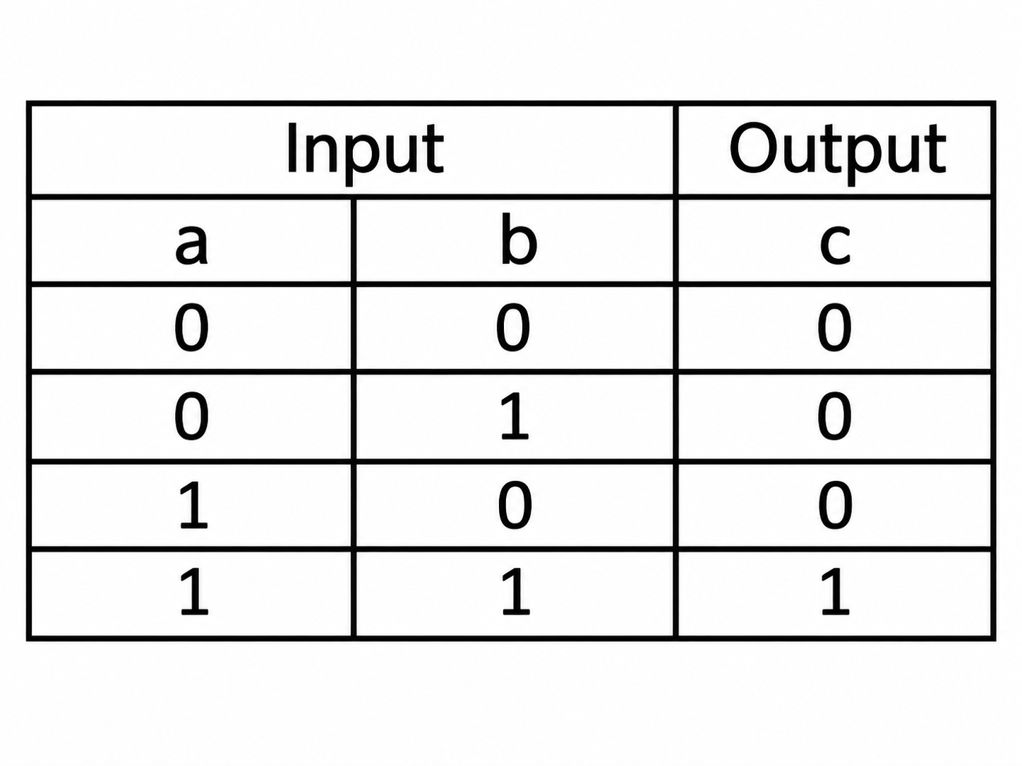
The code is as follows:
1
module top(a, b, c) ;
input a ;
input b ;
output c ;
assign c = a & b ;
endmodule
The testbench is as follows:
1
`timescale 1 ns/1 ns
module top_tb() ;
reg a ;
reg b ;
wire c ;
initial
begin
  a = 0 ;
  b = 0 ;
  forever
  begin
    #({$random}%100)
    a = ~a ;
    #({$random}%100)
    b = ~b ;
  end
end

top t0(.a(a), .b(b),.c(c)) ;

endmodule
The simulation results are as follows:

If the bit width of a and b is greater than 1, for example input [3:0] a and input [3:0] b, then a&b means ANDing the corresponding bits of a and b, such as a[0]&b[0] and a[1]&b[1].
2.5.2 OR Gate
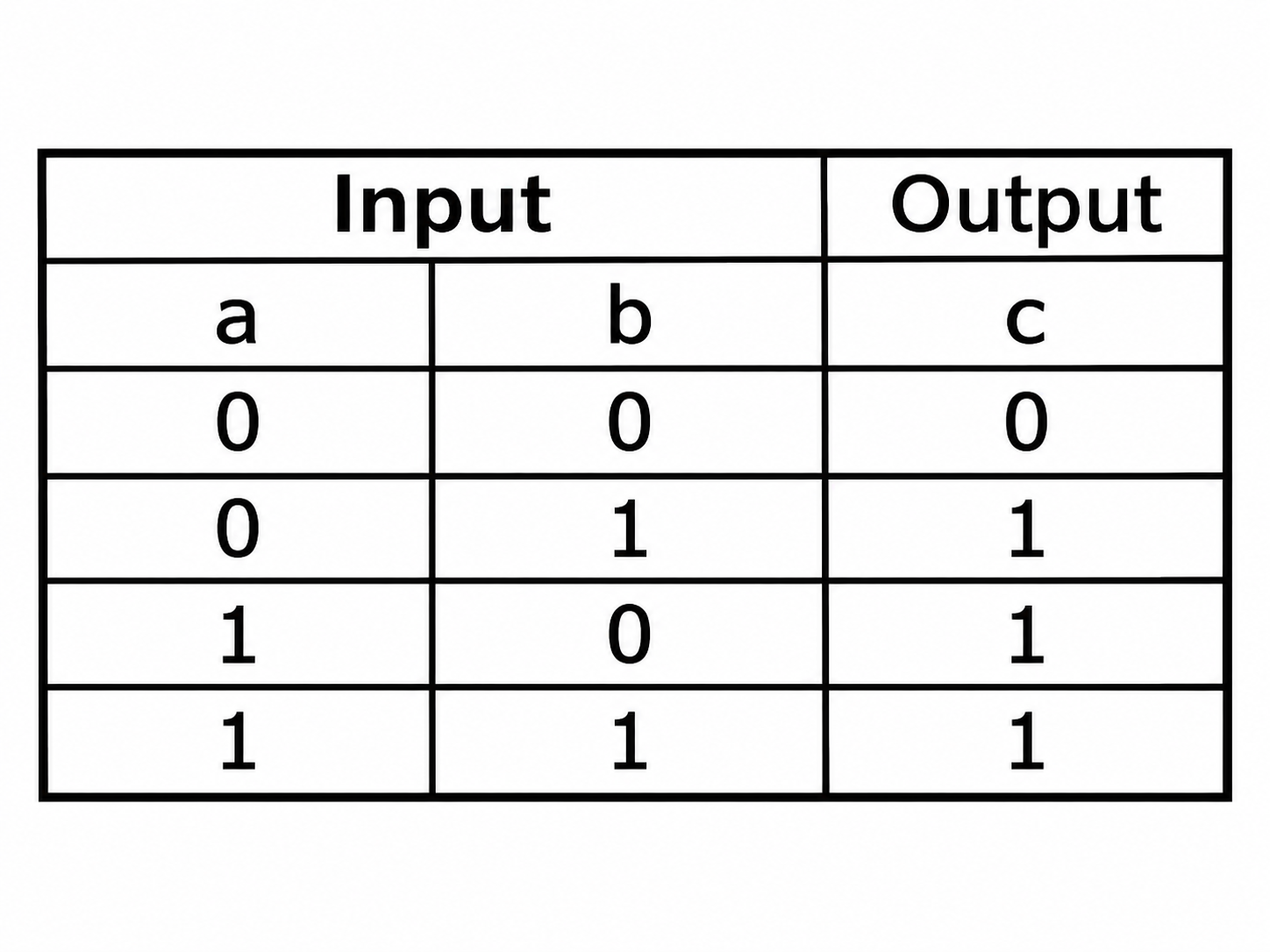
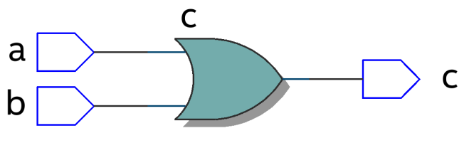
In Verilog, “|” denotes bitwise OR, as in c = a|b. The truth table is shown below: the result is 0 only when both a and b are 0.
The code is as follows:
1
module top(a, b, c) ;
input a ;
input b ;
output c ;
assign c = a \| b ;
endmodule
The testbench is as follows
1
`timescale 1 ns/1 ns
module top_tb() ;
reg a ;
reg b ;
wire c ;
initial
begin
    a = 0 ;
    b = 0 ;
    forever
    begin
        #({$random}%100)
        a = ~a ;
        #({$random}%100)
        b = ~b ;
    end
end

top t0(.a(a), .b(b),.c(c)) ;

endmodule
The simulation results are as follows:

In the same way, when the bit width is greater than 1, it is a bitwise OR.
2.5.3 NOT Gate
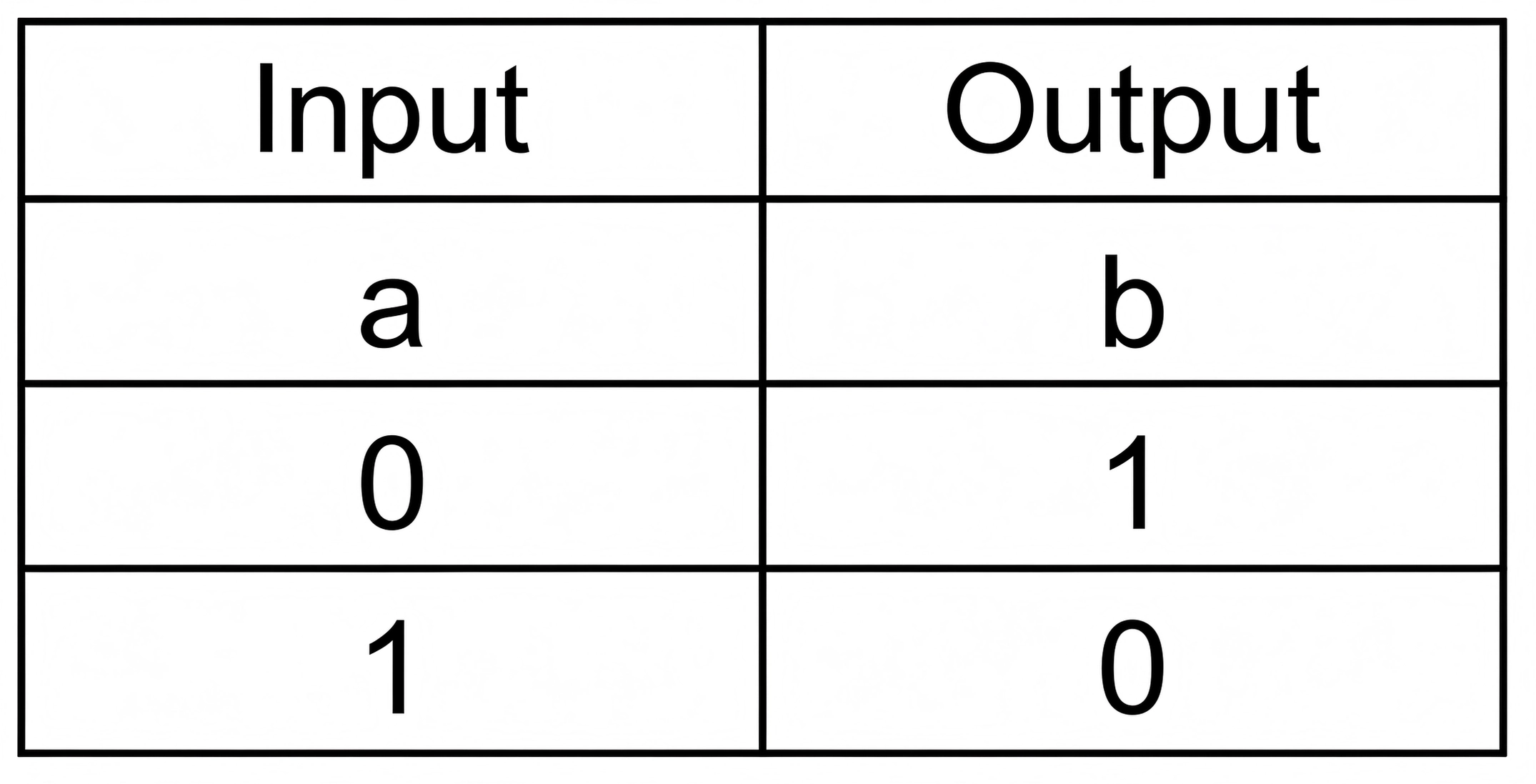
In Verilog, “~” denotes bitwise inversion, as in b=~a. The truth table is shown below: b equals the inverse of a.
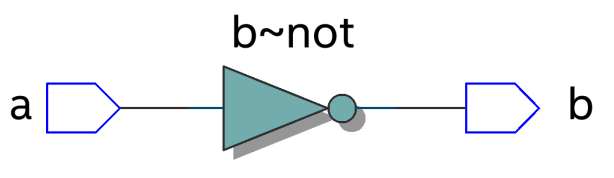
The code is as follows:
1
module top(a, b) ;
input a ;
output b ;
assign b = ~a ;
endmodule
The testbench is as follows:
1
`timescale 1 ns/1 ns
module top_tb() ;
reg a ;
wire b ;

initial
begin
    a = 0 ;
    forever
        begin
        #({$random}%100)
        a = ~a ;
    end
end
top t0(.a(a), .b(b)) ;
endmodule
The simulation results are as follows:

2.5.4 XOR
In Verilog, “^” denotes XOR, as in c= a^b. The truth table is shown below: when a and b are the same, the output is 0.
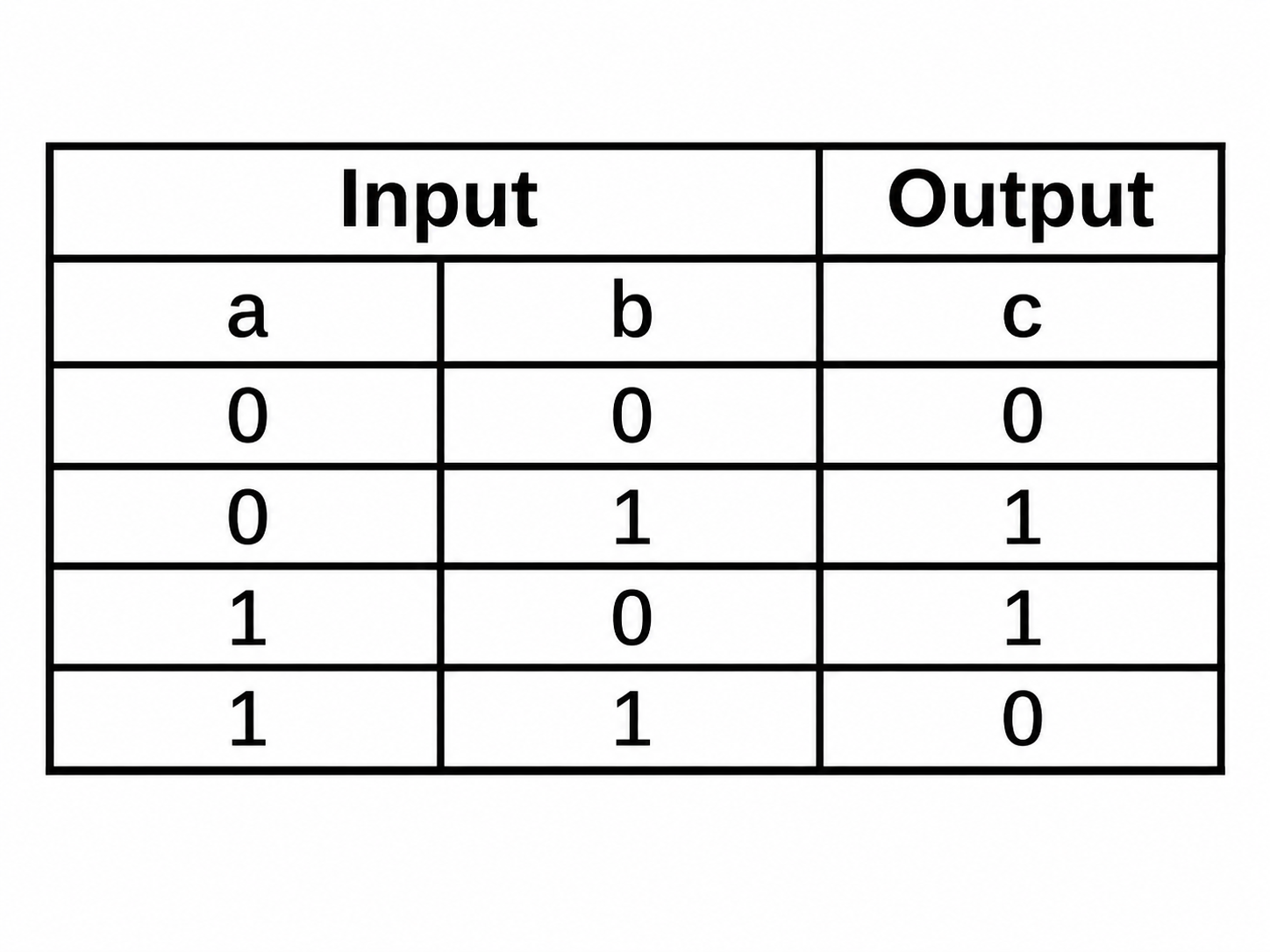
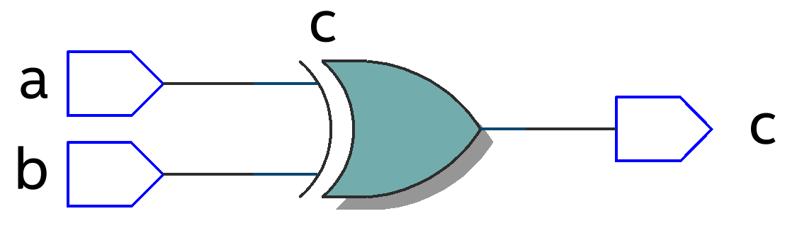
The code is as follows:
1
module top(a, b, c) ;
input a ;
input b ;
output c ;
assign c = a ^ b ;
endmodule
The testbench is as follows:
1
`timescale 1 ns/1 ns
module top_tb() ;
reg a ;
reg b ;
wire c ;
initial
begin
    a = 0 ;
    b = 0 ;
    forever
    begin
        #({$random}%100)
        a = ~a ;
        #({$random}%100)
        b = ~b ;
    end
end
top t0(.a(a), .b(b),.c(c)) ;
endmodule
The simulation results are as follows:

2.5.5 Comparator
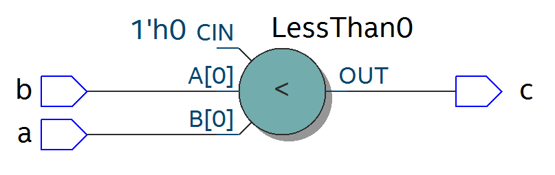
In Verilog these are denoted by greater than “>”, equal to “==”, less than “<”, greater than or equal to “>=”, less than or equal to “<=”, and not equal to “!=”. Taking greater-than as an example, c= a > b ; means that if a is greater than b then the value of c is 1, otherwise it is 0. The truth table is as follows:
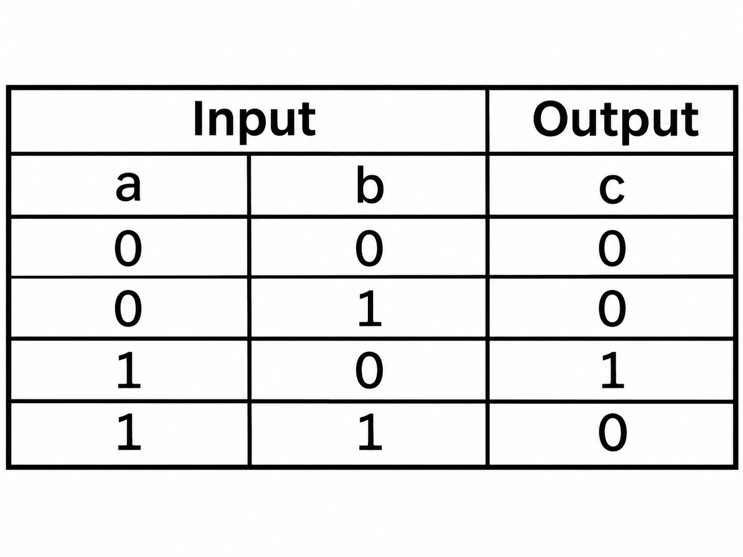
The code is as follows:
1
module top(a, b, c) ;
input a ;
input b ;
output c ;
assign c = a > b ;
endmodule
The testbench is as follows:
1
`timescale 1 ns/1 ns
module top_tb() ;
reg a ;
reg b ;
wire c ;
initial
begin
    a = 0 ;
    b = 0 ;
    forever
    begin
        #({$random}%100)
        a = ~a ;
        #({$random}%100)
        b = ~b ;
    end
end
top t0(.a(a), .b(b),.c(c)) ;
endmodule
The simulation results are as follows:

2.5.6 Half Adder
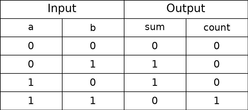
Half adders and full adders are the basic units of arithmetic operation circuits. Because the half adder does not take the carry coming from the lower bit into account, it is called a half adder. sum represents the addition result and count represents the carry. The truth table can be expressed as follows:
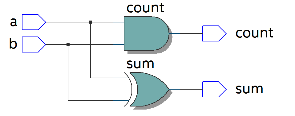
Based on the truth table, the code can be written as follows:
1
module top(a, b, sum, count) ;
input a ;
input b ;
output sum ;
output count ;
assign sum = a ^ b ;
assign count = a & b ;
endmodule
The testbench is as follows:
1
`timescale 1 ns/1 ns
module top_tb() ;
reg a ;
reg b ;
wire sum ;
wire count ;
initial
begin
    a = 0 ;
    b = 0 ;
    forever
    begin
        #({$random}%100)
        a = ~a ;
        #({$random}%100)
        b = ~b ;
    end
end
top t0(.a(a), .b(b),
.sum(sum), .count(count)) ;
endmodule
The simulation results are as follows:

2.5.7 Full Adder
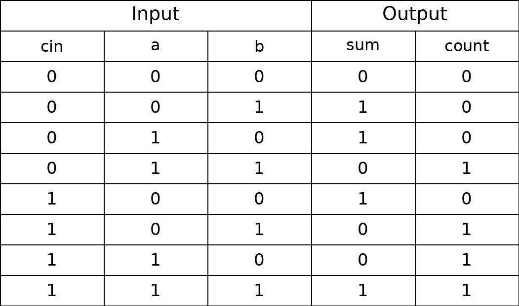
The full adder, by contrast, must also take into account the carry signal cin coming from the lower bit. The truth table is as follows:
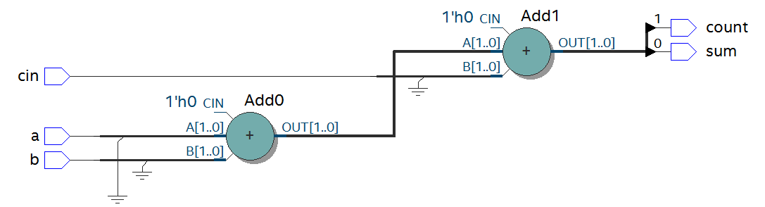
The code is as follows:
1
module top(cin, a, b, sum, count) ;
input cin ;
input a ;
input b ;
output sum ;
output count ;
assign {count,sum} = a + b + cin ;
endmodule
The testbench is as follows:
1
`timescale 1 ns/1 ns
module top_tb() ;
reg a ;
reg b ;
reg cin ;
wire sum ;
wire count ;

initial
begin
    a = 0 ;
    b = 0 ;
    cin = 0 ;
    forever
    begin
        #({$random}%100)
        a = ~a ;
        #({$random}%100)
        b = ~b ;
        #({$random}%100)
        cin = ~cin ;
    end
end
top t0(.cin(cin),.a(a), .b(b),
.sum(sum), .count(count)) ;
endmodule
The simulation results are as follows:

2.5.8 Multiplier
Multiplication is also very simple to express: just use “”, as in ab. The example code is as follows:
1
module top(a, b, c) ;
input [1:0] a ;
input [1:0] b ;
output [3:0] c ;
assign c = a * b ;
endmodule

`timescale 1 ns/1 ns
module top_tb() ;
reg [1:0] a ;
reg [1:0] b ;
wire [3:0] c ;
initial
begin
    a = 0 ;
    b = 0 ;
    forever
    begin
        #({$random}%100)
        a = ~a ;
        #({$random}%100)
        b = ~b ;
    end
end
top t0(.a(a), .b(b),.c(c)) ;
endmodule
The simulation results are as follows:

2.5.9 Multiplexer
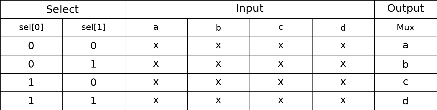
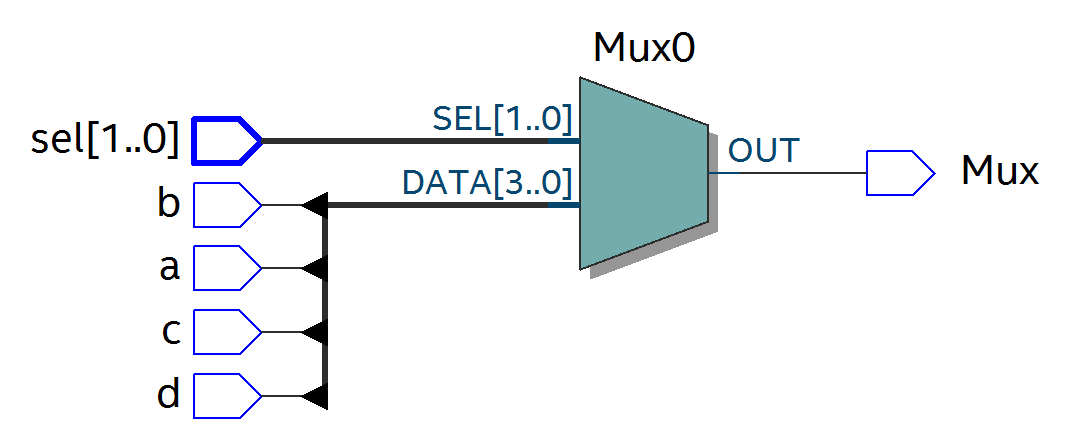
Multiplexers are used very often in Verilog. Through the select signal, different input signals are selected and driven to the output. The truth table below is for a 4-to-1 multiplexer, in which sel[1:0] is the select signal, a, b, c and d are the input signals, and Mux is the output signal.
The code is as follows:
1
module top(a, b, c, d, sel, Mux) ;
input a ;
input b ;
input c ;
input d ;
input [1:0] sel ;
output reg Mux ;

always @(sel or a or b or c or d)
begin
case(sel)
    2'b00 : Mux = a ;
    2'b01 : Mux = b ;
    2'b10 : Mux = c ;
    2'b11 : Mux = d ;
endcase
end
endmodule
The testbench is as follows:
1
`timescale 1 ns/1 ns
module top_tb() ;
reg a ;
reg b ;
reg c ;
reg d ;
reg [1:0] sel ;
wire Mux ;
initial
begin
    a = 0 ;
    b = 0 ;
    c = 0 ;
    d = 0 ;
    forever
    begin
        #({$random}%100)
        a = {$random}%3 ;
        #({$random}%100)
        b = {$random}%3 ;
        #({$random}%100)
        c = {$random}%3 ;
        #({$random}%100)
        d = {$random}%3 ;
    end
end

initial
begin
    sel = 2'b00 ;
    #2000 sel = 2'b01 ;
    #2000 sel = 2'b10 ;
    #2000 sel = 2'b11 ;
end

top t0(.a(a), .b(b),.c(c),.d(d), .sel(sel),.Mux(Mux)) ;
endmodule
The simulation results are as follows

2.5.10 3-to-8 Decoder
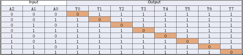
The 3-to-8 decoder is a very commonly used device. Its truth table is shown below; different results are obtained according to the values of A2, A1 and A0.
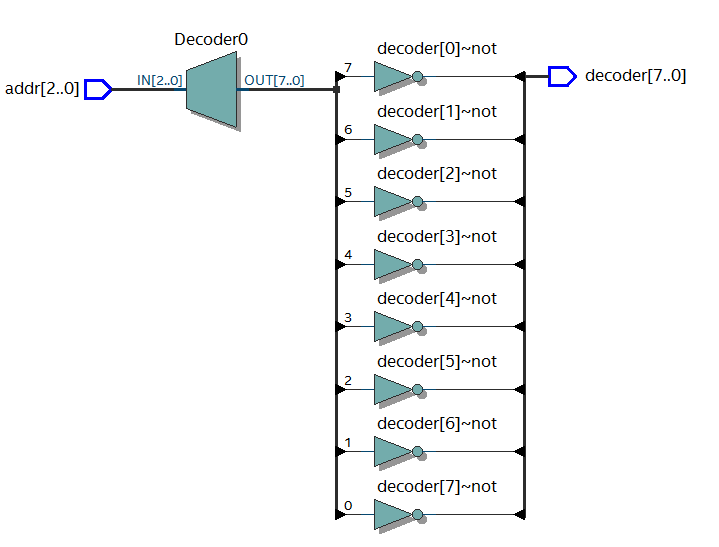
The code is as follows:
1
module top(addr, decoder) ;
input [2:0] addr ;
output reg [7:0] decoder ;
always @(addr)
begin
case(addr)
    3'b000 : decoder = 8'b1111_1110 ;
    3'b001 : decoder = 8'b1111_1101 ;
    3'b010 : decoder = 8'b1111_1011 ;
    3'b011 : decoder = 8'b1111_0111 ;
    3'b100 : decoder = 8'b1110_1111 ;
    3'b101 : decoder = 8'b1101_1111 ;
    3'b110 : decoder = 8'b1011_1111 ;
    3'b111 : decoder = 8'b0111_1111 ;
endcase
end
endmodule
The testbench is as follows:
1
`timescale 1 ns/1 ns
module top_tb() ;
reg [2:0] addr ;
wire [7:0] decoder ;

initial
begin
    addr = 3'b000 ;
    #2000 addr = 3'b001 ;
    #2000 addr = 3'b010 ;
    #2000 addr = 3'b011 ;
    #2000 addr = 3'b100 ;
    #2000 addr = 3'b101 ;
    #2000 addr = 3'b110 ;
    #2000 addr = 3'b111 ;
end
top
t0(.addr(addr),.decoder(decoder)) ;
endmodule
The simulation results are as follows:

2.5.11 Tri-state Buffer
In FPGA applications, bidirectional I/O is often used, and this requires a tri-state buffer, for example bio = en? din: 1’bz ; where en is the enable signal used to turn the tri-state buffer on and off. The RTL diagram below implements bidirectional I/O; refer to the code.

1
module top(en, din, dout, bio) ;
input din ;
input en ;
output dout ;
inout bio ;
assign bio = en? din : 1'bz ;
assign dout = bio ;
endmodule
The testbench connects two bidirectional I/Os to each other.
1
`timescale 1 ns/1 ns
module top_tb() ;
reg en0 ;
reg din0 ;
wire dout0 ;
reg en1 ;
reg din1 ;
wire dout1 ;
wire bio ;

initial
begin
    din0 = 0 ;
    din1 = 0 ;
    forever
    begin
        #({$random}%100)
        din0 = ~din0 ;
        #({$random}%100)
        din1 = ~din1 ;
    end
end

initial
begin
    en0 = 0 ;
    en1 = 1 ;
    #100000
    en0 = 1 ;
    en1 = 0 ;
end

top t0(.en(en0),.din(din0),.dout(dout0),.bio(bio)) ;

top t1(.en(en1),.din(din1),.dout(dout1),.bio(bio)) ;

endmodule
The structure of the testbench is shown in the figure below
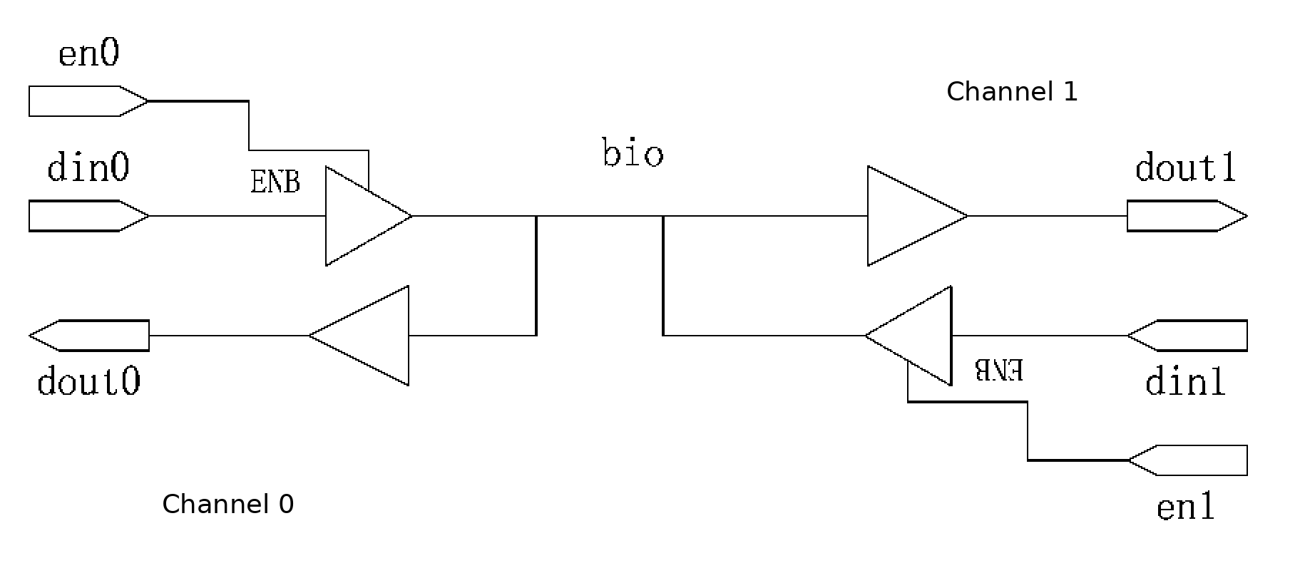
The simulation results are as follows. When en0 is 0 and en1 is 1, channel 1 is enabled, the bidirectional I/O bio equals din1 of channel 1, channel 1 sends data out and channel 0 receives data, and dout0 equals bio. When en0 is 1 and en1 is 0, channel 0 is enabled, bio equals din0 of channel 0, channel 0 sends data out and channel 1 receives data, and dout1 equals bio.

2.6 Sequential Logic
In terms of logic function, the characteristic of a combinational logic circuit is that its output at any moment depends only on the input at that moment and is unrelated to the previous state of the circuit. A sequential logic circuit, by contrast, is characterised in that its output at any moment depends not only on the current input signals but also on the previous state of the circuit. The following analyses typical sequential logic.
2.6.1 D Flip-flop
A D flip-flop stores data on the rising or falling edge of the clock, and its output equals the state of the input signal just before the clock transition.
The code is as follows
1
module top(d, clk, q) ;
input d ;
input clk ;
output reg q ;
always @(posedge clk)
begin
q <= d ;
end
endmodule
The testbench is as follows
1
`timescale 1 ns/1 ns
module top_tb() ;
reg d ;
reg clk ;
wire q ;
initial
begin
    d = 0 ;
    clk = 0 ;
    forever
    begin
        #({$random}%100)
        d = ~d ;
    end
end

always #10 clk = ~clk ;

top t0(.d(d),.clk(clk),.q(q)) ;

endmodule
The RTL diagram is shown below
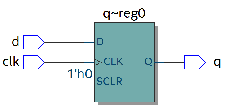
The simulation results are as follows. At time t0 the value of d is 0, so the value of q is also 0; at time t1 d changes, its value becomes 1, and q changes accordingly to 1. It can be seen that within one clock period between t0 and t1, no matter how the value of the input signal d changes, the value of q remains unchanged — that is, it has a storage function, and the stored value is the value of d at the clock transition edge.

2.6.2 Two-stage D Flip-flop
The software performs timing analysis according to the two-stage D flip-flop model. In particular, it is possible to analyse how the data output by the two D flip-flops differs at the same moment. The RTL diagram is as follows:
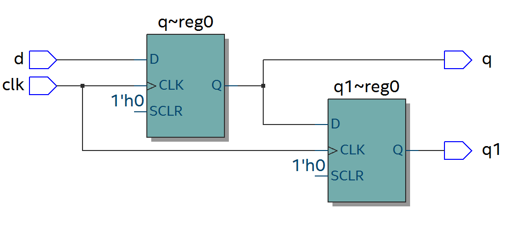
The code is as follows:
1
module top(d, clk, q, q1) ;
input d ;
input clk ;
output reg q ;
output reg q1 ;

always @(posedge clk)
begin
    q <= d ;
end

always @(posedge clk)
begin
    q1 <= q ;
end

endmodule
The testbench is as follows:
1
`timescale 1 ns/1 ns
module top_tb() ;
reg d ;
reg clk ;
wire q ;
wire q1 ;

initial
begin
    d = 0 ;
    clk = 0 ;
    forever
    begin
        #({$random}%100)
        d = ~d ;
    end
end

always #10 clk = ~clk ;

top t0(.d(d),.clk(clk),.q(q),.q1(q1)) ;

endmodule
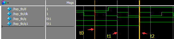
The simulation results are as follows. At time t0, d is 0 and the output q is 0; at time t1, q changes with the data of d, but the value of q before that clock transition is still 0, so q1 is still 0; at time t2, the value of q before the clock transition is 1, so q1 becomes 1 accordingly. q1 lags q by one cycle.
2.6.3 D Flip-flop with Asynchronous Reset
An asynchronous reset is independent of the clock: as soon as the asynchronous reset signal is asserted, the reset operation is triggered. This function is used very often when writing code, to reset and initialise signals. Its RTL diagram is as follows:
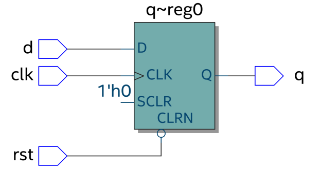
The code is as follows. Note that the asynchronous reset signal must be placed in the sensitivity list: if it is a low-level reset, use negedge; if it is a high-level reset, use posedge.
1
module top(d, rst, clk, q) ;
input d ;
input rst ;
input clk ;
output reg q ;

always @(posedge clk or negedge rst)
begin
    if (rst == 1'b0)
        q <= 0 ;
    else
        q <= d ;
end

endmodule

`timescale 1 ns/1 ns
module top_tb() ;
reg d ;
reg rst ;
reg clk ;
wire q ;

initial
begin
    d = 0 ;
    clk = 0 ;
    forever
    begin
        #({$random}%100)
        d = ~d ;
    end
end

initial
begin
    rst = 0 ;
    #200 rst = 1 ;
end

always #10 clk = ~clk ;

top t0(.d(d),.rst(rst),.clk(clk),.q(q)) ;

endmodule
The simulation results are as follows. Before the reset is released, although the data of the input signal d changes, q is always 0 because the circuit is in the reset state; after the reset, the value of q behaves normally.

2.6.4 D Flip-flop with Asynchronous Reset and Synchronous Clear
As explained above, an asynchronous reset operates independently of the clock, whereas a synchronous clear operates synchronously with the clock signal. Of course it is not limited to a synchronous clear; other synchronous operations are also possible. Its RTL diagram is as follows:
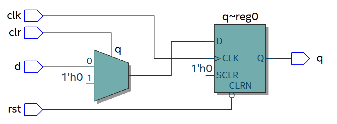
The code is as follows. Unlike an asynchronous reset, a synchronous operation must not place its signal in the sensitivity list.
1
module top(d, rst, clr, clk, q) ;
input d ;
input rst ;
input clr ;
input clk ;
output reg q ;

always @(posedge clk or negedge rst)
begin
    if (rst == 1'b0)
        q <= 0 ;
    else if (clr == 1'b1)
        q <= 0 ;
    else
        q <= d ;
end

endmodule

`timescale 1 ns/1 ns
module top_tb() ;
reg d ;
reg rst ;
reg clr ;
reg clk ;
wire q ;

initial
begin
    d = 0 ;
    clk = 0 ;
    forever
    begin
        #({$random}%100)
        d = ~d ;
    end
end

initial
begin
    rst = 0 ;
    clr = 0 ;
    #200 rst = 1 ;
    #200 clr = 1 ;
    #100 clr = 0 ;
end

always #10 clk = ~clk ;

top t0(.d(d),.rst(rst),.clr(clr),.clk(clk),.q(q)) ;

endmodule
The simulation results are as follows. After the clr signal is pulled high, q is not cleared immediately; the clear operation is performed after the next rising edge of clk, that is, clr is synchronous with clk.

2.6.5 Shift Register
A shift register shifts left or right by one bit on each clock pulse. Because of the characteristics of the D flip-flop, the data output is synchronous with the clock edge. Its structure is as follows: on each clock, the output q of each D flip-flop equals the output value of the preceding D flip-flop, thereby realising the shift function.

Code implementation:
1
module top(d, rst, clk, q) ;
input d ;
input rst ;
input clk ;
output reg [7:0] q ;

always @(posedge clk or negedge rst)
begin
    if (rst == 1'b0)
        q <= 0 ;
    else
        q <= {q[6:0], d} ; //shift left
        //q <= {d, q[7:1]} ; //shift right
end

endmodule
Testbench:
1
`timescale 1 ns/1 ns
module top_tb() ;
reg d ;
reg rst ;
reg clk ;
wire [7:0] q ;

initial
begin
    d = 0 ;
    clk = 0 ;
    forever
    begin
        #({$random}%100)
        d = ~d ;
    end
end

initial
begin
    rst = 0 ;
    #200 rst = 1 ;
end

always #10 clk = ~clk ;

top t0(.d(d),.rst(rst),.clk(clk),.q(q)) ;

endmodule
The simulation results are as follows. After the reset, the data shifts left by one bit on each rising edge of clk.

2.6.6 Single-port RAM
A single-port RAM uses one shared address for both writing and reading. The code is as follows, in which reg [7:0] ram [63:0] means that 64 items of 8-bit data are defined. addr_reg is defined to hold the read address and to send the data out one cycle later.
1
module top
(
input [7:0] data,
input [5:0] addr,
input wr,
input clk,
output [7:0] q
);

reg [7:0] ram[63:0]; //declare ram
reg [5:0] addr_reg; //addr register

always @ (posedge clk)
begin
    if (wr) //write
    ram[addr] <= data;
    addr_reg <= addr;
end

assign q = ram[addr_reg]; //read data

endmodule

`timescale 1 ns/1 ns
module top_tb() ;
reg [7:0] data ;
reg [5:0] addr ;
reg wr ;
reg clk ;
wire [7:0] q ;

initial
begin
    data = 0 ;
    addr = 0 ;
    wr = 1 ;
    clk = 0 ;
end

always #10 clk = ~clk ;

always @(posedge clk)
begin
    data <= data + 1'b1 ;
    addr <= addr + 1'b1 ;
end

top t0
(.data(data),
.addr(addr),
.clk(clk),
.wr(wr),
.q(q)) ;

endmodule
The simulation results are as follows; the output q is consistent with the data written.

2.6.7 Simple Dual Port RAM
In a simple dual-port RAM the read and write addresses are independent, so the write or read address can be selected at random and read and write operations can be performed at the same time. The code is as follows; in the testbench an enable signal is defined and the read address is driven when it is asserted.
1
module top
(
input [7:0] data,
input [5:0] write_addr,
input [5:0] read_addr,
input wr,
input rd,
input clk,
output reg [7:0] q
);

reg [7:0] ram[63:0]; //declare ram
reg [5:0] addr_reg; //addr register

always @ (posedge clk)
begin
    if (wr) //write
        ram[write_addr] <= data;
    if (rd) //read
        q <= ram[read_addr];
end

endmodule

`timescale 1 ns/1 ns
module top_tb() ;
reg [7:0] data ;
reg [5:0] write_addr ;
reg [5:0] read_addr ;
reg wr ;
reg clk ;
reg rd ;
wire [7:0] q ;

initial
begin
    data = 0 ;
    write_addr = 0 ;
    read_addr = 0 ;
    wr = 0 ;
    rd = 0 ;
    clk = 0 ;
    #100 wr = 1 ;
    #20 rd = 1 ;
end
always #10 clk = ~clk ;

always @(posedge clk)
begin
    if (wr)
    begin
        data <= data + 1'b1 ;
        write_addr <= write_addr + 1'b1 ;
        if (rd)
            read_addr <= read_addr + 1'b1 ;
    end
end

top t0
(.data(data),
.write_addr(write_addr),
.read_addr(read_addr),
.clk(clk),
.wr(wr),
.rd(rd),
.q(q)) ;

endmodule
The simulation results are as follows; when rd is asserted, the read address is driven and the data is read out.

2.6.8 True Dual Port RAM
A true dual-port RAM has two sets of control lines and data lines, allowing two systems to read from and write to it. The code is as follows:
1
module top
(
input [7:0] data_a, data_b,
input [5:0] addr_a, addr_b,
input wr_a, wr_b,
input rd_a, rd_b,
input clk,
output reg [7:0] q_a, q_b
);

reg [7:0] ram[63:0]; //declare ram

//Port A
always @ (posedge clk)
begin
    if (wr_a) //write
    begin
        ram[addr_a] <= data_a;
        q_a <= data_a ;
    end
    if (rd_a)
    //read
        q_a <= ram[addr_a];
end

//Port B
always @ (posedge clk)
begin
    if (wr_b) //write
    begin
        ram[addr_b] <= data_b;
        q_b <= data_b ;
    end
    if (rd_b)
    //read
        q_b <= ram[addr_b];
end

endmodule

`timescale 1 ns/1 ns
module top_tb() ;
reg [7:0] data_a, data_b ;
reg [5:0] addr_a, addr_b ;
reg wr_a, wr_b ;
reg rd_a, rd_b ;
reg clk ;
wire [7:0] q_a, q_b ;

initial
begin
    data_a = 0 ;
    data_b = 0 ;
    addr_a = 0 ;
    addr_b = 0 ;
    wr_a = 0 ;
    wr_b = 0 ;
    rd_a = 0 ;
    rd_b = 0 ;
    clk = 0 ;
    #100 wr_a = 1 ;
    #100 rd_b = 1 ;
end

always #10 clk = ~clk ;

always @(posedge clk)
begin
    if (wr_a)
    begin
        data_a <= data_a + 1'b1 ;
        addr_a <= addr_a + 1'b1 ;
    end
    else
    begin
        data_a <= 0 ;
        addr_a <= 0 ;
    end
end

always @(posedge clk)
begin
    if (rd_b)
    begin
        addr_b <= addr_b + 1'b1 ;
    end
    else addr_b <= 0 ;
end

top
t0(.data_a(data_a), .data_b(data_b),
.addr_a(addr_a), .addr_b(addr_b),
.wr_a(wr_a), .wr_b(wr_b),
.rd_a(rd_a), .rd_b(rd_b),
.clk(clk),
.q_a(q_a), .q_b(q_b)) ;
endmodule
The simulation results are as follows

2.6.9 Single-port ROM
ROM is used to store data. A ROM can be initialised in the code form shown below, but this method becomes rather cumbersome for a large-capacity ROM; it is recommended to implement the ROM with the ROM IP core provided by the FPGA and to add an initialisation file.
Code implementation Testbench
1
module top
(
input [3:0] addr,
input clk,
output reg [7:0] q
);

always @(posedge clk)
begin
case(addr)
    4'd0 : q <= 8'd15 ;
    4'd1 : q <= 8'd24 ;
    4'd2 : q <= 8'd100 ;
    4'd3 : q <= 8'd78 ;
    4'd4 : q <= 8'd98 ;
    4'd5 : q <= 8'd105 ;
    4'd6 : q <= 8'd86 ;
    4'd7 : q <= 8'd254 ;
    4'd8 : q <= 8'd76 ;
    4'd9 : q <= 8'd35 ;
    4'd10 : q <= 8'd120 ;
    4'd11 : q <= 8'd85 ;
    4'd12 : q <= 8'd37 ;
    4'd13 : q <= 8'd19 ;
    4'd14 : q <= 8'd22 ;
    4'd15 : q <= 8'd67 ;
    default: q <= 8'd0 ;
endcase
end

endmodule

`timescale 1 ns/1 ns
module top_tb() ;
reg [3:0] addr ;
reg clk ;
wire [7:0] q ;

initial
begin
    addr = 0 ;
    clk = 0 ;
end

always #10 clk = ~clk ;

always @(posedge clk)
begin
    addr <= addr + 1'b1 ;
end

top t0(.addr(addr),
.clk(clk),
.q(q)) ;
endmodule
The simulation results are as follows

2.6.10 Finite State Machine
Finite state machines are used very often in Verilog to handle relatively complex logic: different states are defined, and according to trigger conditions the machine jumps to the corresponding state and performs the corresponding processing in each state. Finite state machines mainly use always and case statements. The following gives an example of a four-state finite state machine.
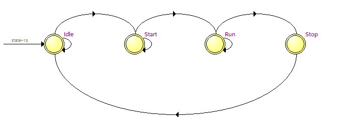
An 8-bit shift register is designed in the program. In the Idle state, it checks whether the shift_start signal is high; if it is high, it enters the Start state. In the Start state it delays for 100 cycles and then enters the Run state, where the shift operation is performed. If the shift_stop signal is asserted, it enters the Stop state; in the Stop state it clears the value of q and then jumps back to the Idle state.
In a Mealy finite state machine the output depends not only on the current state but also on the input signals, so in the RTL it is connected to the input signals.
1
module top
(
input shift_start,
input shift_stop,
input rst,
input clk,
input d,
output reg [7:0] q
);

parameter Idle = 2'd0 ; //Idle state
parameter Start = 2'd1 ; //Start state
parameter Run = 2'd2 ; //Run state
parameter Stop = 2'd3 ; //Stop state

reg [1:0] state ; //statement
reg [4:0] delay_cnt ; //delay counter

always @(posedge clk or negedge rst)
begin
    if (!rst)
    begin
        state <= Idle ;
        delay_cnt <= 0 ;
        q <= 0 ;
    end
    else
    case(state)
    Idle : begin
        if (shift_start)
        state <= Start ;
    end
    Start : begin
        if (delay_cnt == 5'd99)
        begin
            delay_cnt <= 0 ;
            state <= Run ;
        end
        else
            delay_cnt <= delay_cnt + 1'b1 ;
    end
    Run : begin
        if (shift_stop)
            state <= Stop ;
        else
            q <= {q[6:0], d} ;
    end
    Stop : begin
        q <= 0 ;
        state <= Idle ;
    end
    default: state <= Idle ;
    endcase
end

endmodule
In a Moore finite state machine the output depends only on the current state and has nothing to do with the input signals; the input signals only affect state transitions and do not affect the output. For example, the handling of delay_cnt and q depends only on the state.
1
module top
(
input shift_start,
input shift_stop,
input rst,
input clk,
input d,
output reg [7:0] q
);

parameter Idle = 2'd0 ; //Idle state
parameter Start = 2'd1 ; //Start state
parameter Run = 2'd2 ; //Run state
parameter Stop = 2'd3 ; //Stop state

reg [1:0] current_state ; //statement
reg [1:0] next_state ;
reg [4:0] delay_cnt ; //delay counter
//First part: statement transition

always @(posedge clk or negedge rst)
begin
if (!rst)
    current_state <= Idle ;
else
    current_state <= next_state ;
end

//Second part: combination logic, judge statement transition condition

always @(*)
begin
    case(current_state)
    Idle : begin
        if (shift_start)
            next_state <= Start ;
        else
            next_state <= Idle ;
    end
    Start : begin
        if (delay_cnt == 5'd99)
            next_state <= Run ;
        else
            next_state <= Start ;
    end
    Run : begin
        if (shift_stop)
            next_state <= Stop ;
        else
            next_state <= Run ;
    end
    Stop : next_state <= Idle ;
    default: next_state <= Idle ;
    endcase
end

//Last part: output data

always @(posedge clk or negedge rst)
begin
    if (!rst)
        delay_cnt <= 0 ;
    else if (current_state == Start)
        delay_cnt <= delay_cnt + 1'b1 ;
    else
        delay_cnt <= 0 ;
end

always @(posedge clk or negedge rst)
begin
    if (!rst)
        q <= 0 ;
    else if (current_state == Run)
        q <= {q[6:0], d} ;
    else
        q <= 0 ;
end

endmodule
The two programs above use two different styles of coding. The first, the Mealy state machine, uses the one-segment style with only a single always statement: all state transitions, the evaluation of state transition conditions and the data output are inside one always statement. The drawback is that if there are too many states, the whole program becomes lengthy. The second, the Moore state machine, uses the three-segment style: one always statement for the state transition, one always statement as combinational logic to evaluate the state transition conditions, and a separate always statement for the data output. This style is more intuitive and clearer, and does not become cumbersome even with many states.
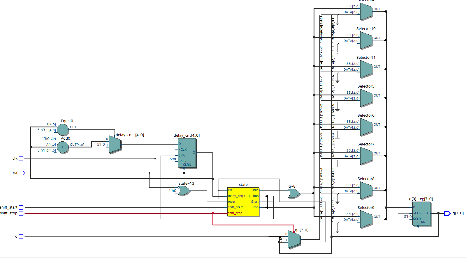
RTL diagram of the Mealy finite state machine
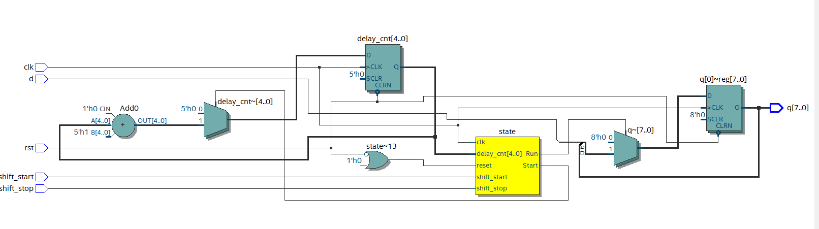
RTL diagram of the Moore finite state machine
The testbench is as follows:
1
`timescale 1 ns/1 ns
module top_tb() ;

reg shift_start ;
reg shift_stop ;
reg rst ;
reg clk ;
reg d ;
wire [7:0] q ;

initial
begin
    rst = 0 ;
    clk = 0 ;
    d = 0 ;
    #200 rst = 1 ;
    forever
    begin
        #({$random}%100)
        d = ~d ;
    end
end

initial
begin
    shift_start = 0 ;
    shift_stop = 0 ;
    #300 shift_start = 1 ;
    #1000 shift_start = 0 ;
    shift_stop = 1 ;
    #50 shift_stop = 0 ;
end

always #10 clk = ~clk ;

top t0
(
.shift_start(shift_start),
.shift_stop(shift_stop),
.rst(rst),
.clk(clk),
.d(d),
.q(q)
);

endmodule
The simulation results are as follows:

2.7 Summary
This document has introduced the modules commonly used in combinational logic and sequential logic. Among them the finite state machine is relatively complex but is used very often. Readers are encouraged to understand it deeply, to use it more in their code and to think about it more, which is conducive to improving their level quickly.
Chapter 3 The PL "Hello World" LED Experiment
The Vivado project for this experiment is “led”.
For ZYNQ, PL (FPGA) development is crucial. This is also where ZYNQ has an advantage over other ARM devices: many ARM-side peripherals can be customised. Before customising ARM-side peripherals, let us first use an LED example to become familiar with the PL (FPGA) development flow and the basic operations of the Vivado software. This development flow is exactly the same as that of an FPGA chip without an ARM core.
In this example we perform an LED control experiment: the LED on the development board is toggled once every second, giving the sequence on, off, on, off. Once you can control an LED, you will gradually be able to control other peripherals as well.
3.1 LED Hardware Introduction
1. One red user LED is connected to the PL part of the development board. This one LED is controlled entirely by the PL.
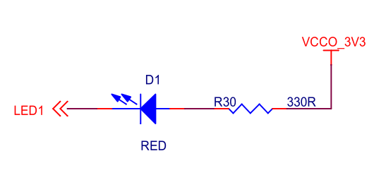
2. We can determine the binding relationship between the LED and the PL pins from the wiring in the schematic.
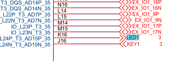
The corresponding pin information
3. In the schematic, all IOs whose names start with PS_MIO are PS-side IOs; they do not need to be constrained, and indeed cannot be constrained.
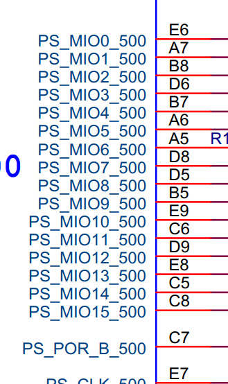
3.2 Creating the Vivado Project
1. Start Vivado. Under Windows this can be done by double-clicking the Vivado shortcut.

2. In the Vivado development environment, click “Create New Project” to create a new project.
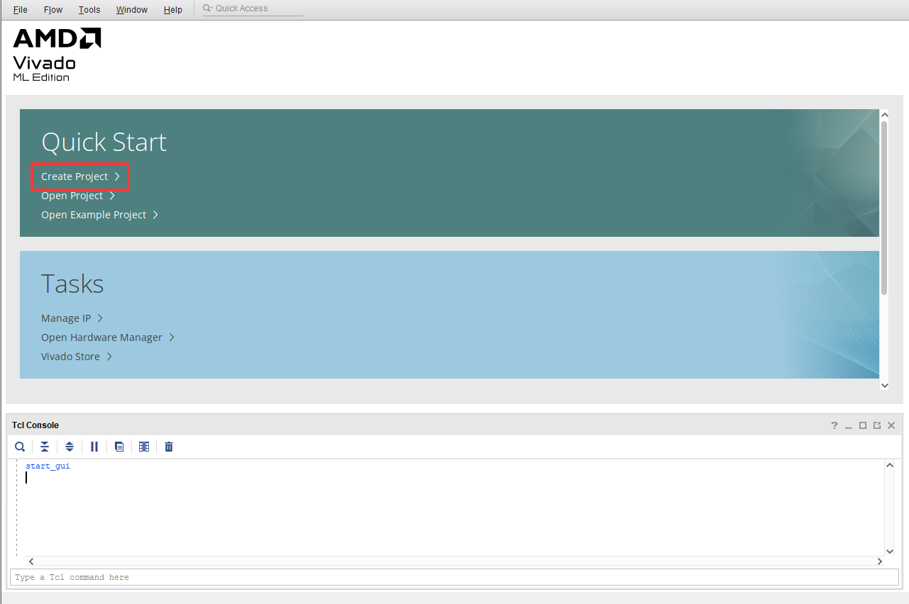
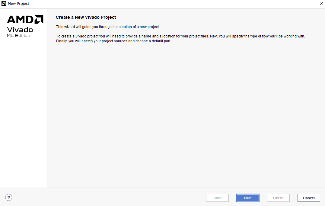
3. A wizard for creating a new project pops up; click “Next”.
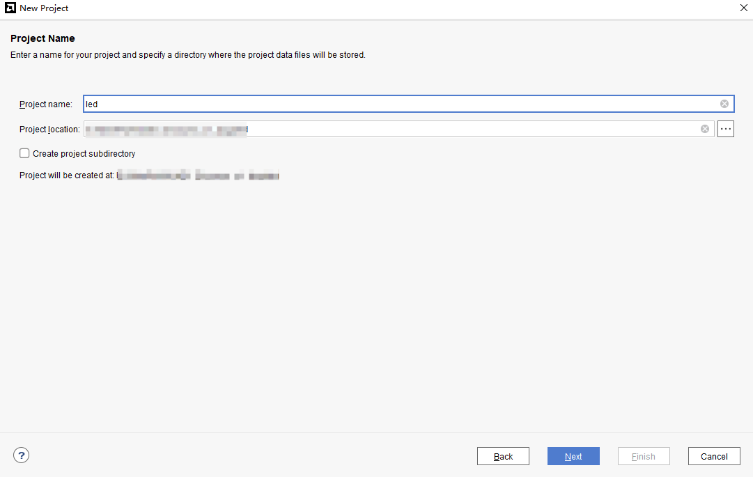
4. In the dialog box that appears, enter the project name and the directory where the project is to be stored; here we use led as the project name. Note that the project path (“Project location”) must not contain Chinese characters or spaces, and the path name must not be too long.
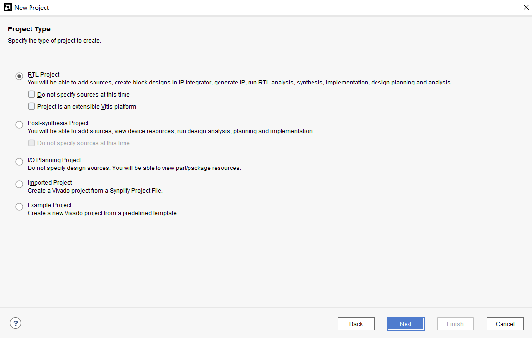
5. For the project type, select “RTL Project”.
6. For “Target language” select “Verilog”. Although Verilog is selected, VHDL can also be used; mixed-language design is supported.
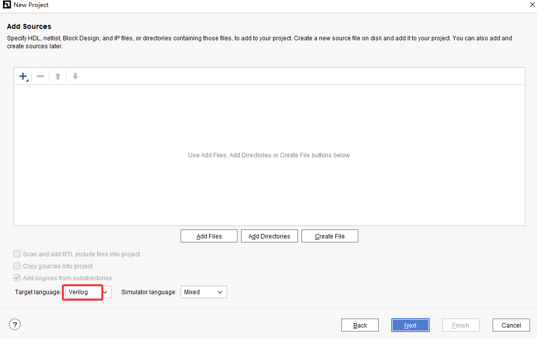
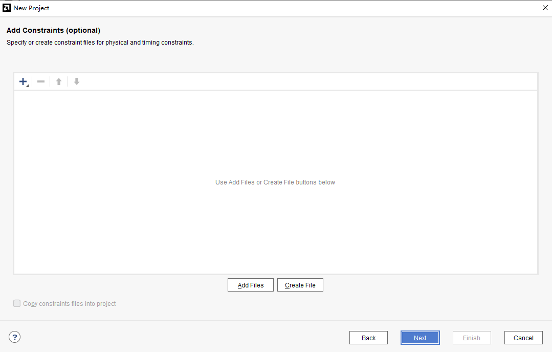
7. Click “Next” without adding any files.
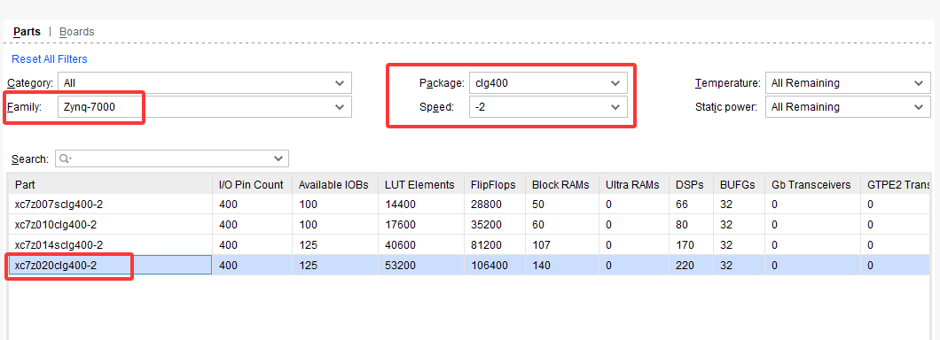
8. In the “Part” options, select “Zynq-7000” for the device family “Family”. For the PI-ZN010-F1-1 development board, select “clg400” for “Package” and “-1” for Speed to narrow the selection range. Select “xc7z010clg400-1” from the drop-down list. “-1” indicates the speed grade: the larger the number, the better the performance, and a chip with a higher speed grade is downward compatible with chips of lower speed grades.
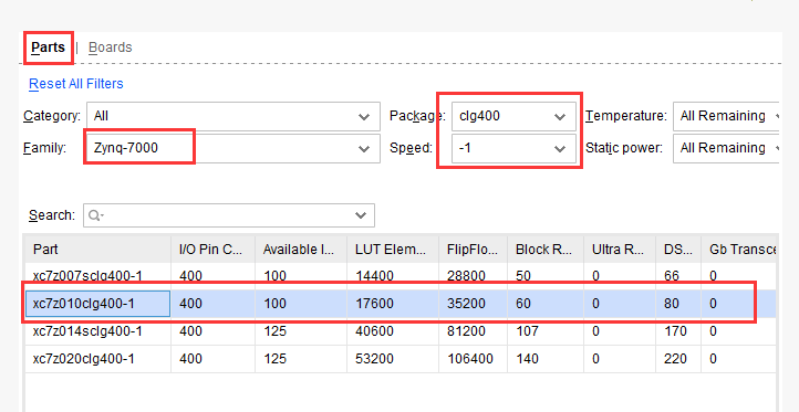
For the PI-ZN020-F1-1 development board, select “clg400” for “Package” and “-2” for Speed to narrow the selection range. Select “xc7z020clg400-2” from the drop-down list.
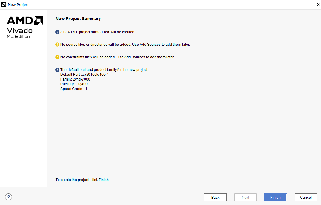
9. Click “Finish” to complete the creation of the project named “led”.
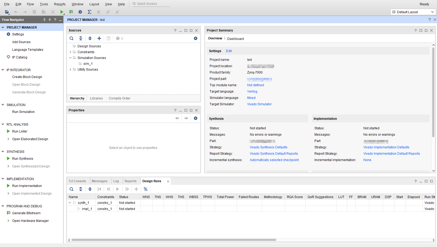
10. The Vivado software interface
3.3 Creating a Verilog HDL File to Light the LED
1. Click the Add Sources icon under Project Manager (or use the shortcut Alt+A).
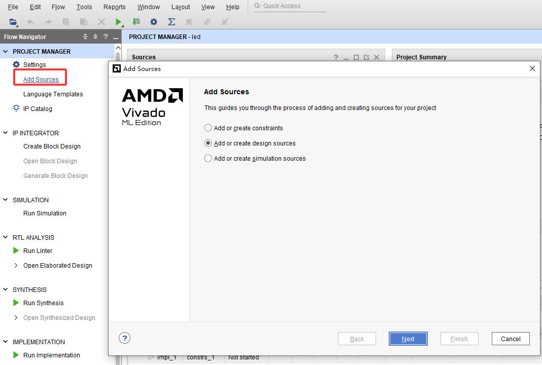
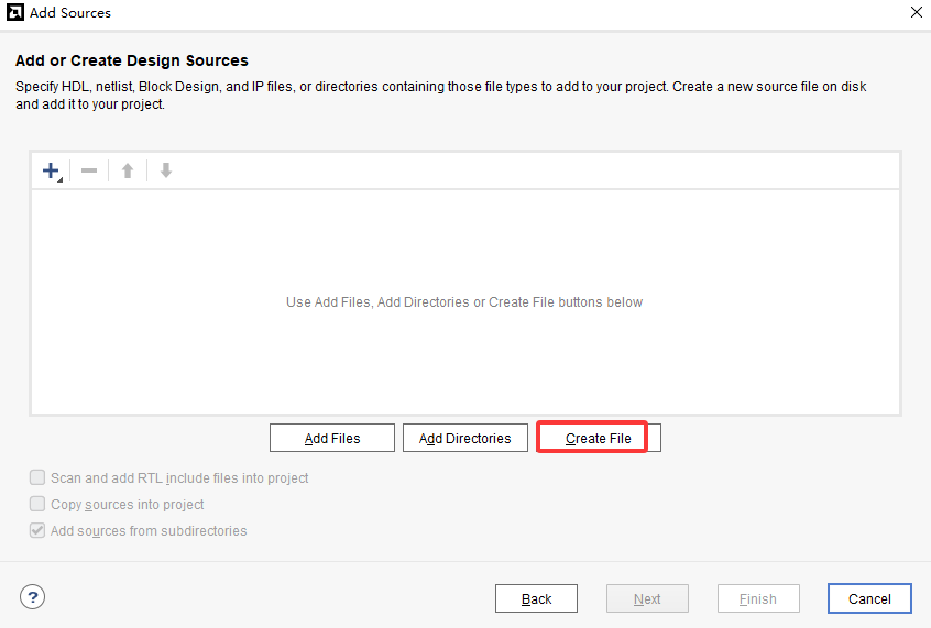
2. Select “Create File” to create a file.
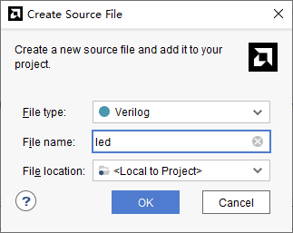
3. Set “File name” to “led” and click “OK”.
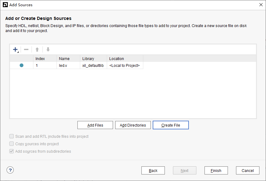
4. Click “Finish” to complete the addition of the “led.v” file.
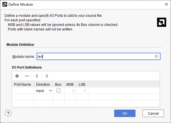
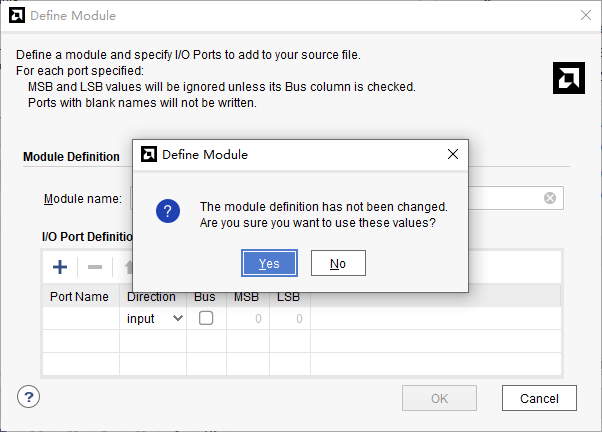
5. In the “Define Module” dialog box that pops up, you can specify the module name (“Module name”) of the “led.v” file; here leave the default “led”. You can also specify some ports; for now none are specified. Click “OK”.
6. Select “Yes” in the dialog box that pops up.
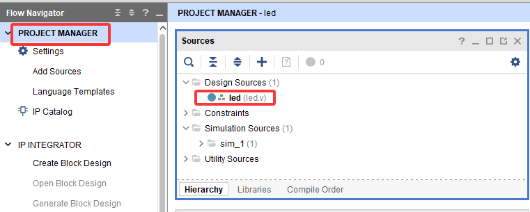
7. Double-click “led.v” to open the file and then edit it.
8. Write “led.v”. A 32-bit register timer is defined here to count repeatedly from 0 to 49999999 (1 second). When the count reaches 49999999 (1 second), the register timer becomes 0 and the LED is toggled. In this way, if the LED was originally off it will be lit, and if it was originally on it will go off. The code after writing is as follows:
1
module led(
    input sys_clk,
    input rst_n,
    output reg led
);

reg[31:0] timer_cnt;

always@(posedge sys_clk or negedge rst_n)
begin
    if (!rst_n)
    begin
        led <= 1'b0 ;
        timer_cnt <= 32'd0 ;
        end
    else if(timer_cnt >= 32'd49_999_999)
    begin
        led <= ~led;
        timer_cnt <= 32'd0;
    end
    else
    begin
        led <= led;
        timer_cnt <= timer_cnt + 32'd1;
    end
end

endmodule
9. Save the file after writing the code.
3.4 Adding Pin Constraints
The constraint file format used by Vivado is the xdc file. An xdc file mainly contains pin constraints, clock constraints and group constraints. Here we need to assign the input and output ports in the led.v program to real pins on the FPGA.
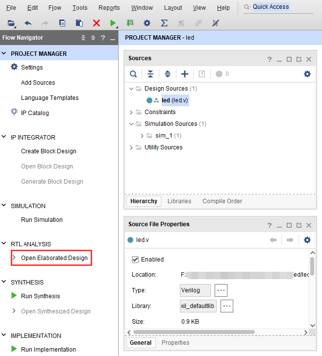
1. Click “Open Elaborated Design”.
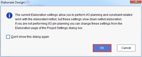
2. Click the “OK” button in the window that pops up.
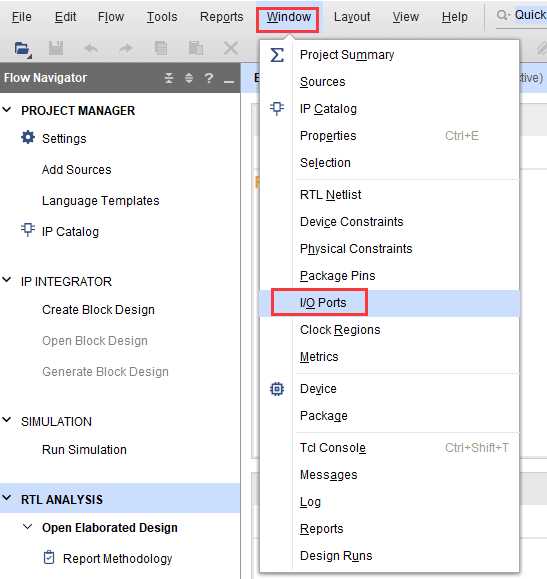
3. In the menu, select “Window -> I/O Ports”.
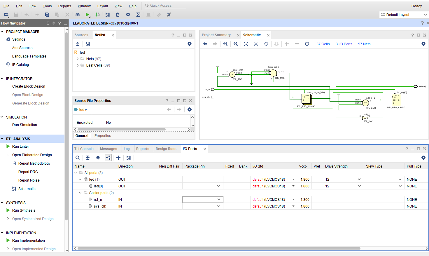
4. In the I/O Ports window that pops up, you can see the pin assignment.
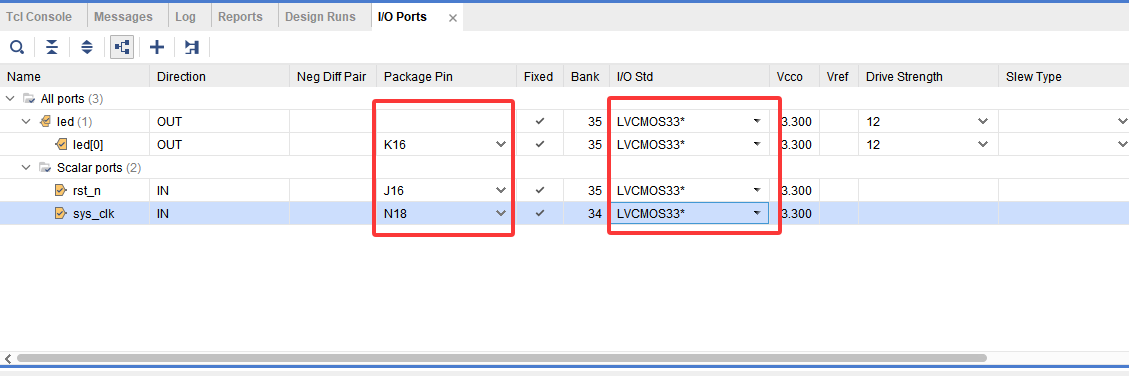
5. Bind the reset signal rst_n to the PL-side push button, assign pins and I/O standards to the LED and the clock, and click the save icon when done.
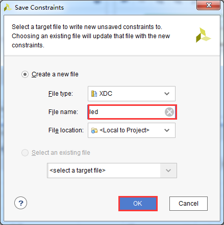
6. A window pops up asking to save the constraint file; we fill in “led” as the file name, leave the file type at the default “XDC”, and click “OK”.
7. Open the “led.xdc” file just generated; you can see that it is a Tcl script. If we understand this syntax, we can constrain the pins entirely by writing the led.xdc file ourselves.
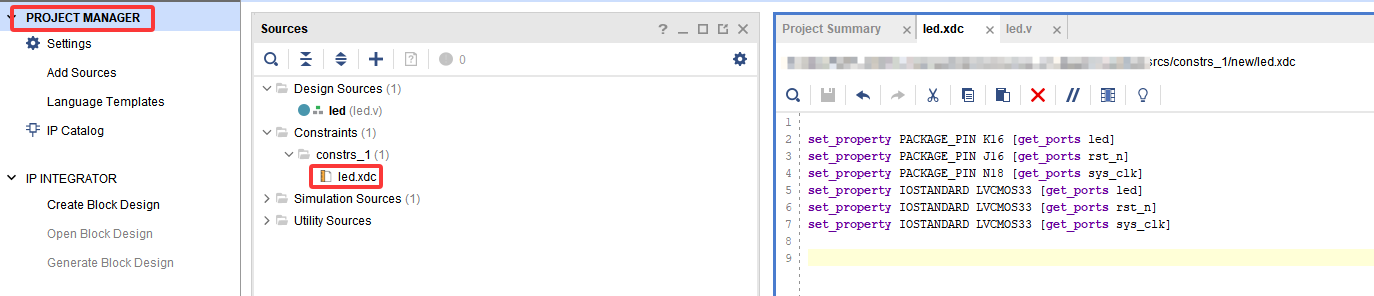
Below we introduce the most basic XDC syntax. For an ordinary IO, only the pin number and the voltage need to be constrained. The pin constraint is as follows:
set_property PACKAGE_PIN "pin number" [get_ports “port name”]
The level standard is constrained as follows:
set_property IOSTANDARD "I/O standard" [get_ports “port name”]
Note here that the text is case-sensitive. If the port name is an array, enclose it in { }; the port name must be identical to the name in the source code, and port names must not be the same as keywords.
In an I/O standard, the number after “LVCMOS33” refers to the voltage of the FPGA bank. The bank in which the LED is located is 3.3 V, so the I/O standard is “LVCMOS33”. Vivado by default requires a correct I/O standard and pin number to be assigned to every IO.
3.5 Adding Timing Constraints
Besides pin assignment, an FPGA design has another important constraint: timing constraints. Here we demonstrate how to create a timing constraint by means of the wizard.
1. Click “Run Synthesis” to start synthesis.
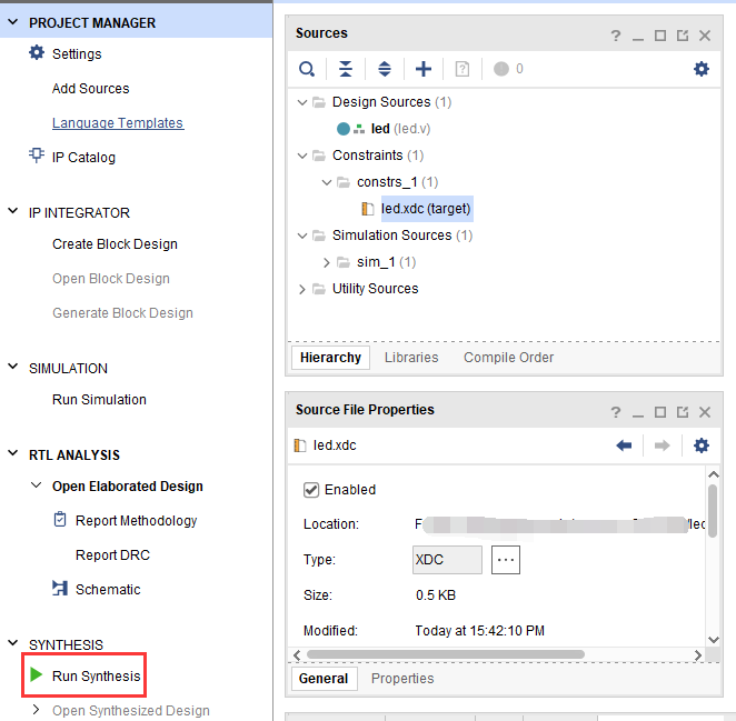
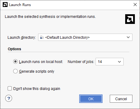
2. In the dialog box that pops up, click “OK”.
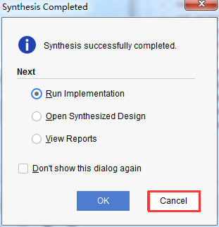
3. When synthesis is complete, click “Cancel”.
4. Click “Constraints Wizard”.
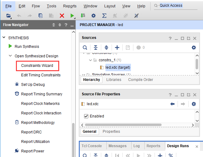
5. In the window that pops up, click “Next”.

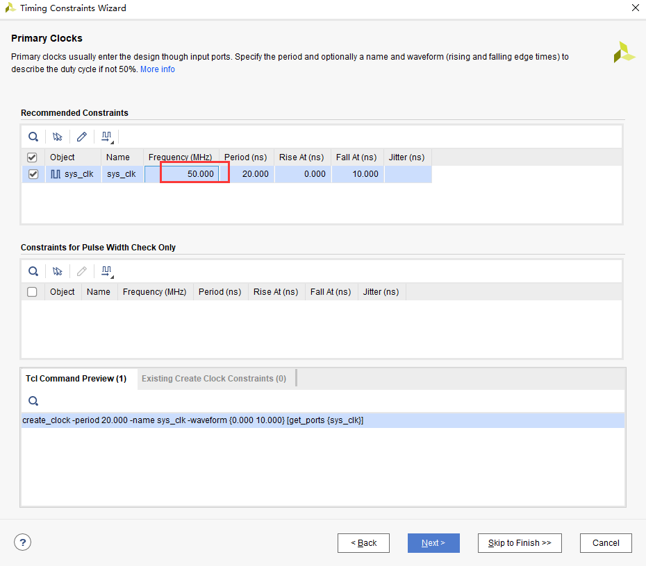
6. The timing constraints wizard identifies the clocks in the design. Here set the frequency of “sys_clk” to 50MHz, then click “Skip to Finish” to end the timing constraints wizard.
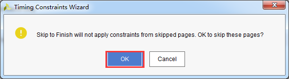
7. In the window that pops up, click “OK”.
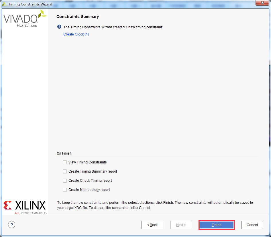
8. Click “Finish”.
9. At this point the led.xdc file has been updated. Click “Reload” to reload the file, and save the file.
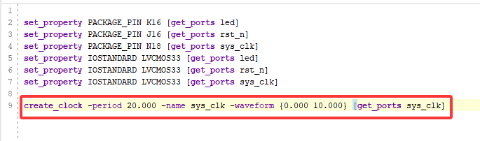
3.6 Generating the BIT File
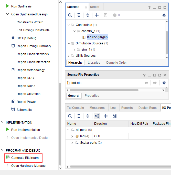
1. The compilation process can be subdivided into synthesis, place and route, bit file generation and so on. Here we directly click “Generate Bitstream” to generate the bit file.
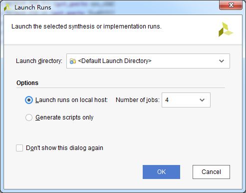
2. In the dialog box that pops up, you can select the number of jobs; this is related to the number of CPU cores, and generally the larger the number, the faster the compilation. Click “OK”.
3. Compilation now starts; you can see a status message in the upper right corner. During compilation the run may be intercepted by antivirus software or a PC manager utility, which can make it impossible to compile or make it fail to compile successfully for a long time.

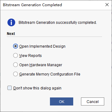
4. There are no errors during compilation and compilation completes. A dialog box pops up asking us to choose the next action; you can select “Open Hardware Manager”, and of course you can also select “Cancel”. Here we select “Cancel” and do not download yet.
3.7 Vivado Simulation
Next, let us try our hand at using the simulation tool built into Vivado to output waveforms and verify whether the results of the running-light program design agree with our expectations (note: you can also simulate before generating the bit file). The specific steps are as follows:
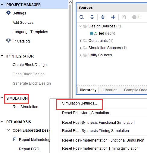
1. Set up the Vivado simulation configuration by right-clicking Simulation Settings under SIMULATION.
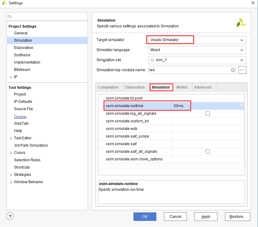
2. Configure as shown in the Simulation Settings window below. Here it is set to 50ms (set it according to your own needs); leave the other settings at their defaults and click OK to finish.
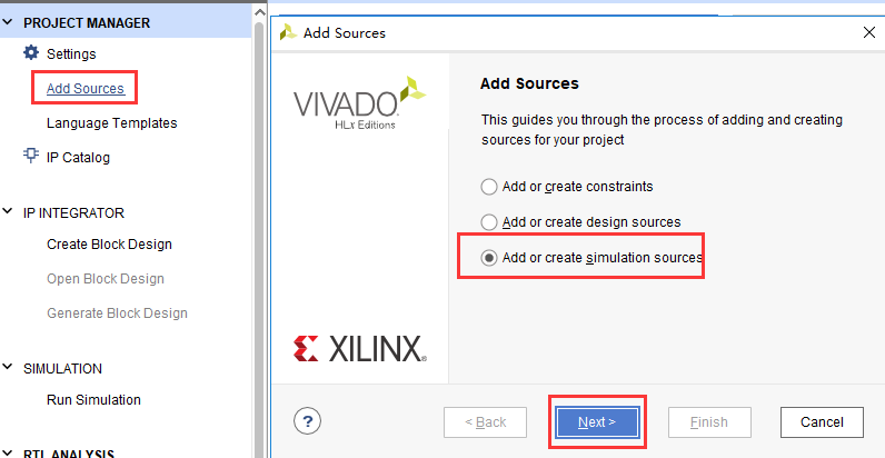
3. Add a stimulus test file: click the Add Sources icon under Project Manager, make the settings shown below and then click Next.
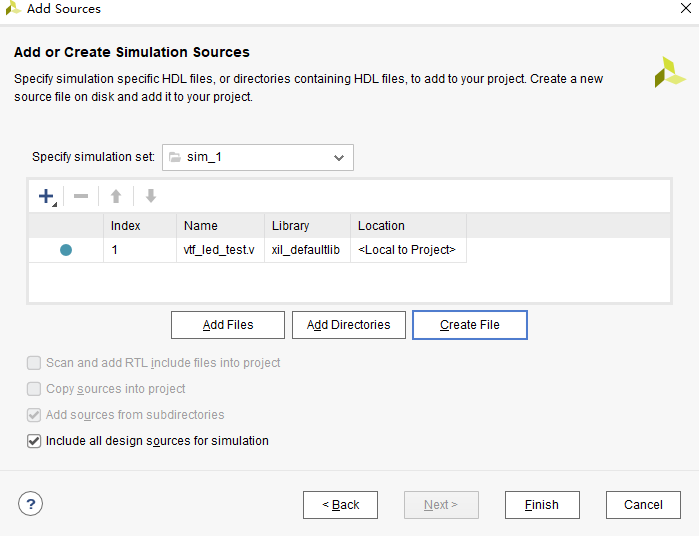
4. Click Create File to generate the simulation stimulus file.
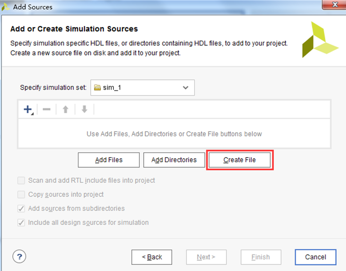
In the dialog box that pops up, enter the name of the stimulus file; here we enter the name vtf_led_test.
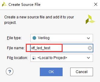
5. Click the Finish button to return.
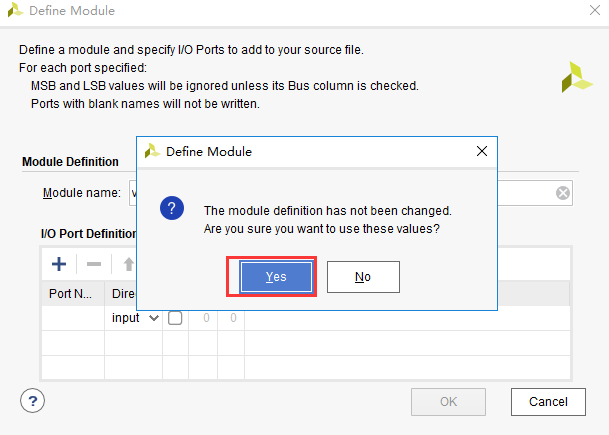
For now we do not add IO Ports; click OK.
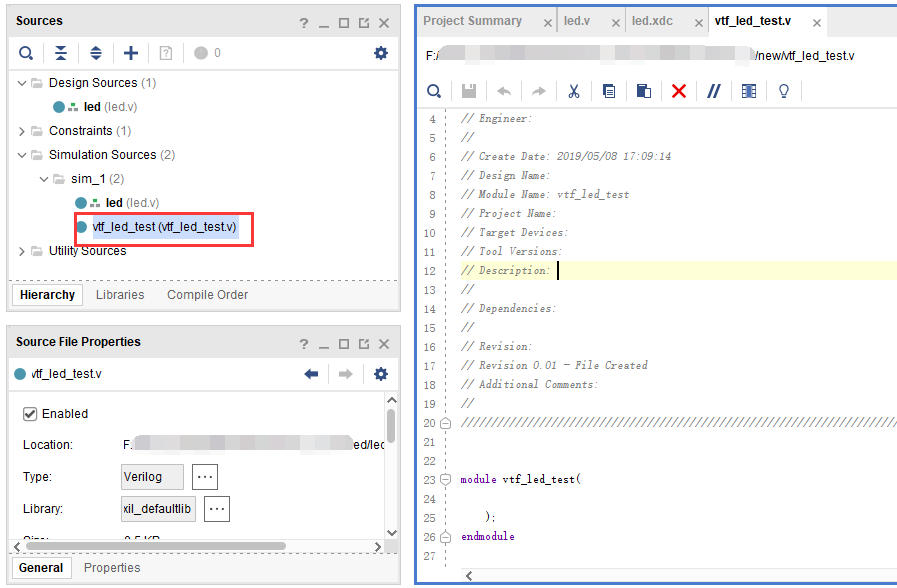
In the Simulation Sources directory there is now the vtf_led_test file just added. Double-click to open it; you can see that it contains only the module name definition and nothing else.
6. Next we need to write the contents of this vtf_led_test.v file. First define the input and output signals, then instantiate the led_test module so that the led_test program becomes part of this test program. Then add the reset and clock stimuli. The completed vtf_led_test.v file is as follows:
1
`timescale 1ns / 1ps
//////////////////////////////////////////////////////////////////////////////////
// Module Name: vtf_led_test
//////////////////////////////////////////////////////////////////////////////////
module vtf_led_test;
// Inputs
reg sys_clk;
reg rst_n ;
// Outputs
wire led;

// Instantiate the Unit Under Test (UUT)
led uut (
    .sys_clk(sys_clk),
    .rst_n(rst_n),
    .led(led)
);

initial
begin
    // Initialize Inputs
    sys_clk = 0;
    rst_n = 0 ;
    #1000 ;
    rst_n = 1;
end

//Create clock
always #10 sys_clk = ~ sys_clk;

endmodule
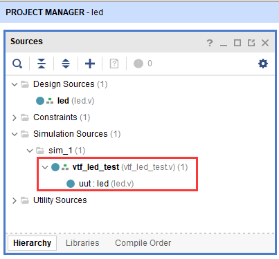
7. Save after writing. vtf_led_test.v automatically becomes the top level of this simulation hierarchy, with the design file led_test.v below it.
8. Click the Run Simulation button and then select Run Behavioral Simulation. A behavioural simulation is sufficient here.
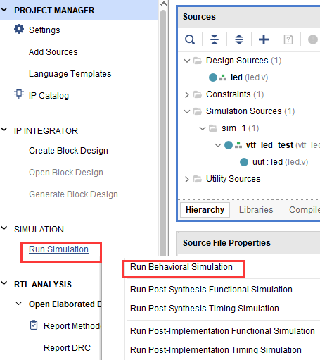
If there are no errors, the simulation software in Vivado starts working.
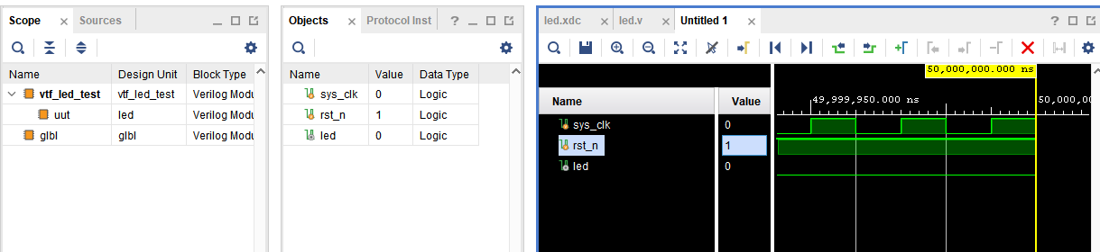
9. After the simulation interface appears it looks as shown below; the interface shows the waveform after the simulation software automatically runs to the 50ms set in the simulation configuration.
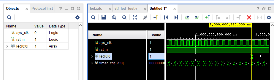
Because the state of LED[0:0] changes slowly in the program design and simulation is time-consuming, observe the change of the timer[31:0] counter here. Add it to the Wave window for observation (click uut under the Scope pane, then right-click timer under the Objects pane and select Add Wave Window in the drop-down menu that appears).
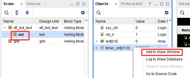
After adding it, timer is displayed in the Wave waveform pane, as shown in the figure below.

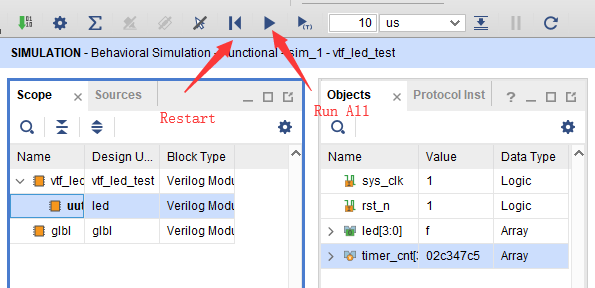
10. Click the Restart button marked below to reset, then click the Run All button. (Patience is required!) You can see that the simulation waveform matches the design. (Note: the longer the simulation runs, the more disk space the simulation waveform file occupies; the waveform file is in the xx.sim folder in the project directory.)
3.8 Download
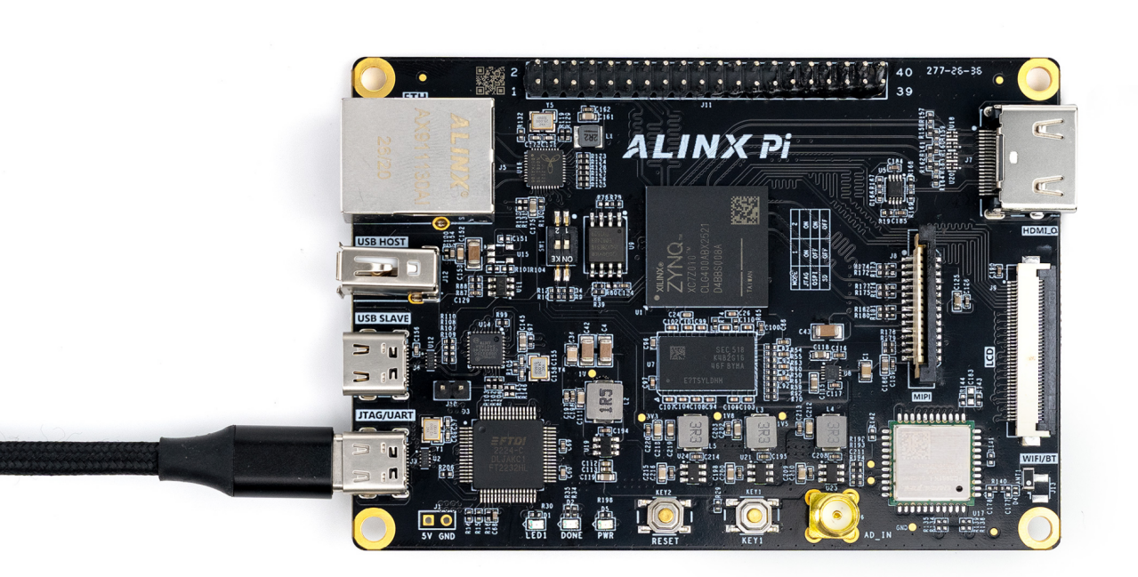
1. Connect the JTAG interface of the development board and power on the development board.
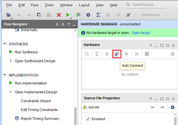
2. In the “HARDWARE MANAGER” interface, click “Auto Connect” to connect to the device automatically.
3. You can see that JTAG has detected the ARM and FPGA cores.
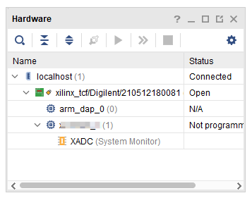
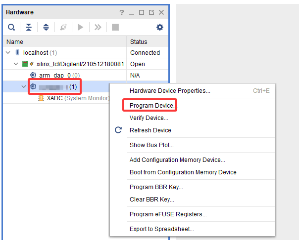
4. Select xc7z010_1, right-click and choose “Program Device...”.
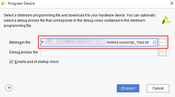
5. Click “Program” in the window that pops up.
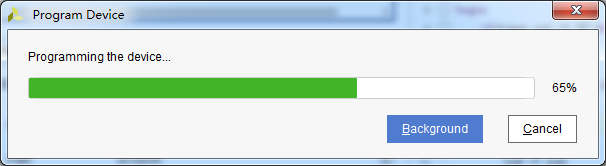
6. Wait for the download.
7. After the download completes, we can see the 4 LEDs starting to change once per second. At this point the simple Vivado flow has been experienced. Later chapters will explain that programming the program into the Flash requires the cooperation of the PS system; a PL-only project cannot program the Flash directly. This is described in the FAQ section of the chapter “Experiencing the ARM, Bare-metal Output of ‘Hello World’”.
3.9 Online Debugging
Simulation and download have been described above, but simulation does not require the program to be programmed into the board and is a rather idealised result. Below we introduce the Vivado online debugging method to observe changes in internal signals. Vivado has a built-in logic analyser called ILA, which can be used to observe changes in internal signals online and is very helpful for debugging. In this experiment we observe the changes of the timer_cnt and led signals.
3.9.1 Adding the ILA IP Core
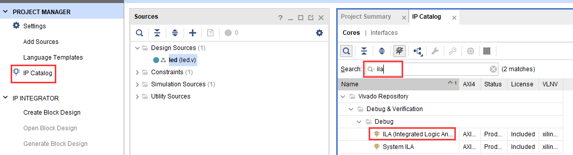
1. Click IP Catalog, search for ila in the search box, and double-click the ILA IP.
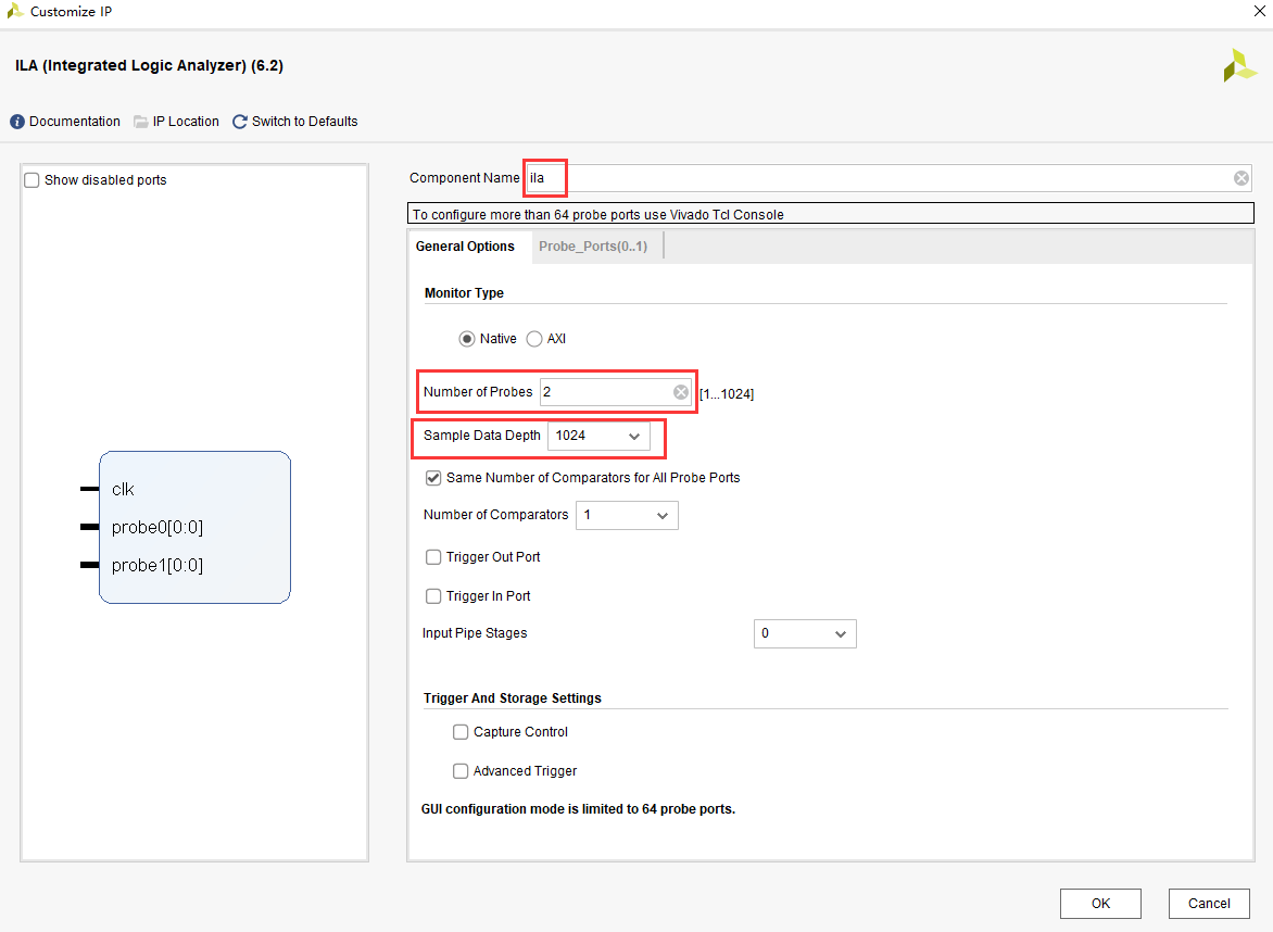
2. Change the name to ila. Since two signals are to be sampled, set the number of Probes to 2. Sample Data Depth refers to the sampling depth: the higher the setting, the more signals are captured, and likewise the more resources are consumed.
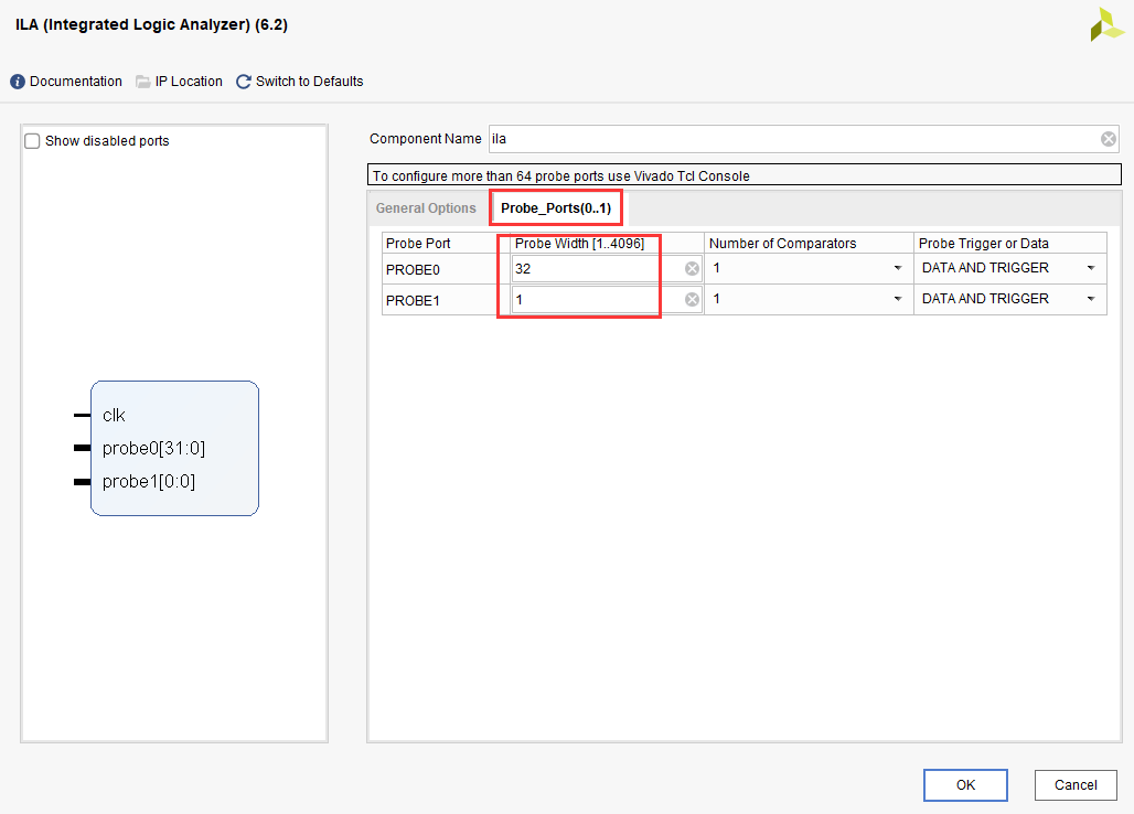
3. On the Probe_Ports page, set the width of the probes: set the width of PROBE0 to 32 for sampling timer_cnt, and the width of PROBE1 to 1 for sampling led. Click OK.
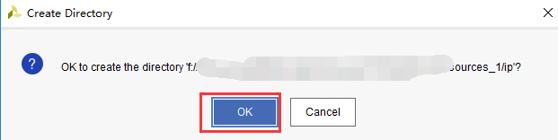
A window pops up; select OK.
Then make the settings shown below and click Generate.
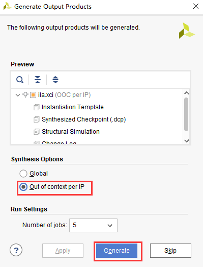
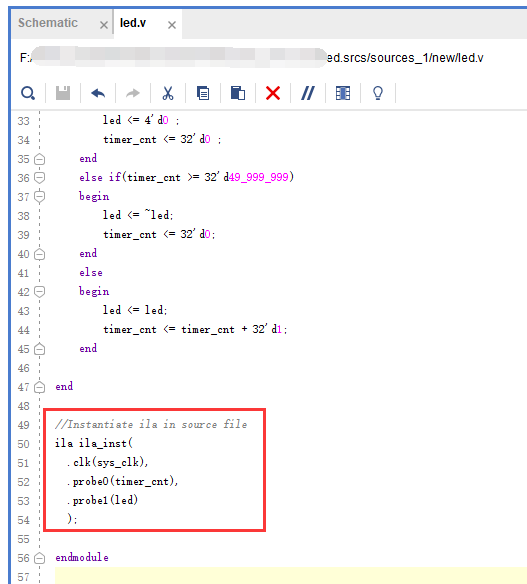
4. Instantiate ila in led.v and save.
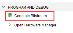
5. Regenerate the Bitstream.
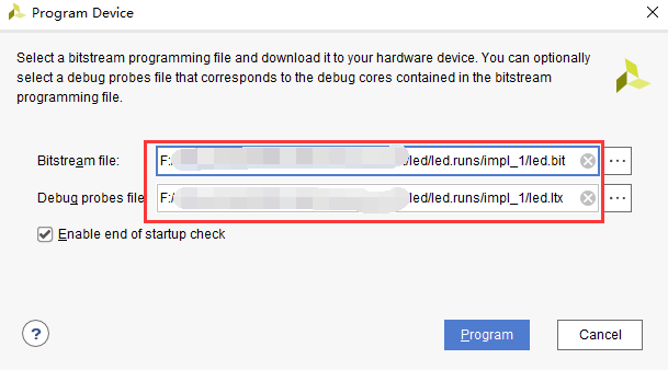
6. Download the program. At this point you will see the bit and ltx files; click program.
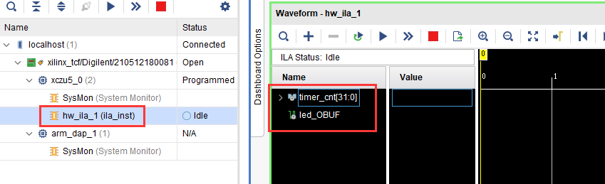
7. The online debugging window now pops up, showing the signals we added.
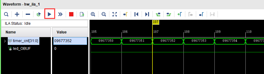
Click the Run button and the signal data appears.
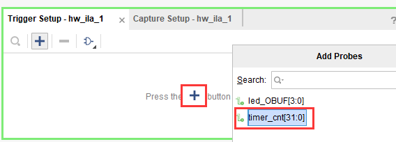
You can also use triggered capture: click “+” in the Trigger Setup window and select the timer_cnt signal.
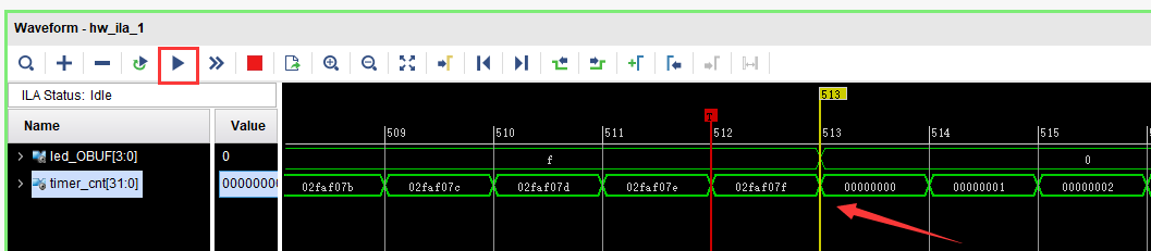
Change Radix to U, that is, decimal, and set Value to 49999999, which is the maximum value counted by timer_cnt.

Click Run again and you can see that the trigger succeeded; timer_cnt is now displayed in hexadecimal, and led toggles at this moment.
3.9.2 MARK DEBUG
The method of adding an ILA IP for online debugging was described above. Below we describe adding synthesis attributes in the code to achieve online debugging.
1. First open led.v and comment out the instantiation of ila.
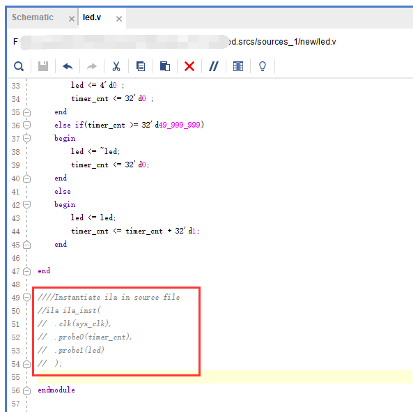
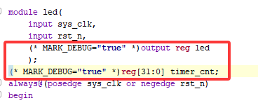
2. Add ( MARK_DEBUG=”true” ) in front of the definitions of led and timer_cnt, and save the file.
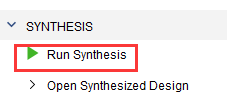
3. Click Synthesize.
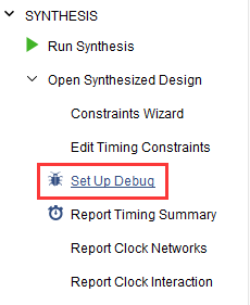
4. When synthesis is finished, click Set Up Debug.
5. Click Next in the window that pops up.
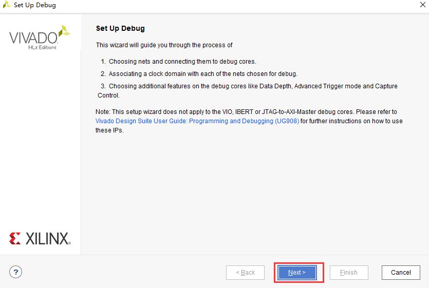
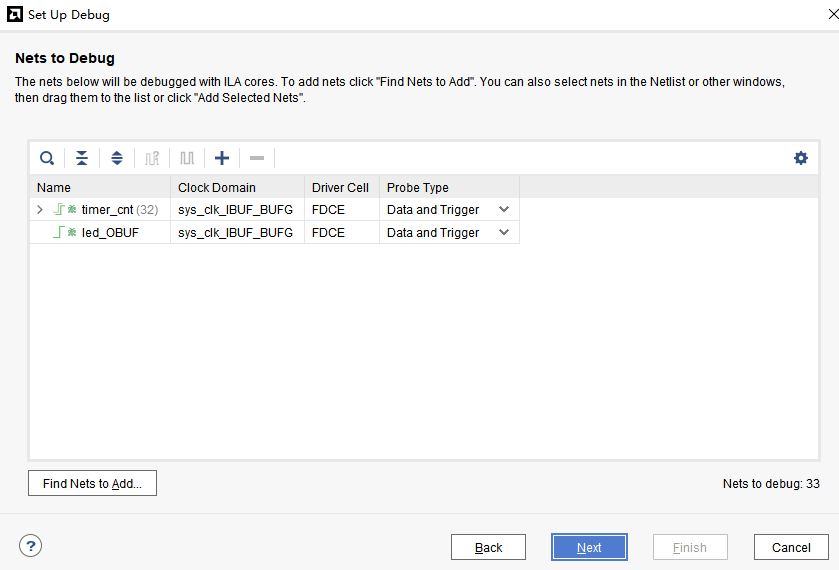
Click Next with the default settings.
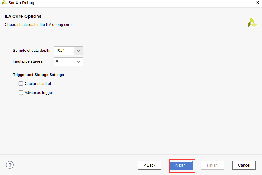
In the sampling depth window, select Next.
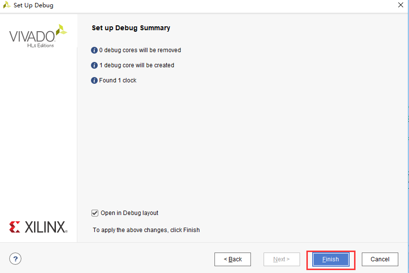
Click Finish.
Click Save.
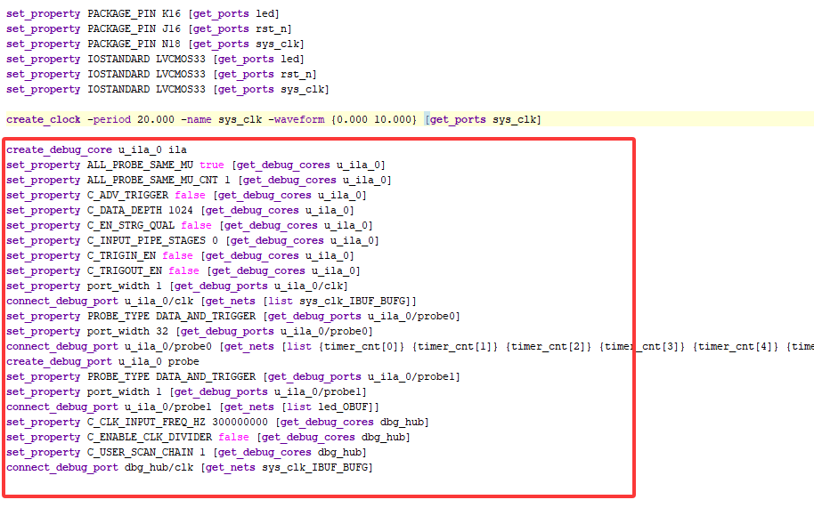
The constraints for the added ila core can now be seen in the xdc file.
5. Regenerate the bitstream.
6. The debugging method is the same as before and is not repeated here.
3.10 Experiment Summary
This chapter has introduced how to develop a program on the PL side, including project creation, constraints, simulation and online debugging. This method can be referenced in subsequent code development approaches.
Chapter 4 FPGA On-chip RAM Read/Write Test Experiment
The Vivado project for this experiment is “ram_test”.
RAM is a basic module commonly used in FPGA and can be widely used to cache data; it is also the basis of ROM and FIFO. This experiment introduces how to use the RAM inside the FPGA and how a program reads from and writes to that RAM.
4.1 Experiment Principle
Xilinx already provides a RAM IP core in VIVADO. We only need to instantiate a RAM through the IP core, then write and read the data stored in the RAM according to the RAM read/write timing. In the experiment, through the online logic analyser ila integrated in VIVADO, we can observe the RAM read/write timing and the data read from the RAM.
4.2 Creating the Vivado Project
Before adding the RAM IP, first create a project named ram_test, then add the RAM IP to the project, as follows:
1. Click IP Catalog as shown below, search for ram in the pane that pops up on the right, find Block Memory Generator and double-click it.
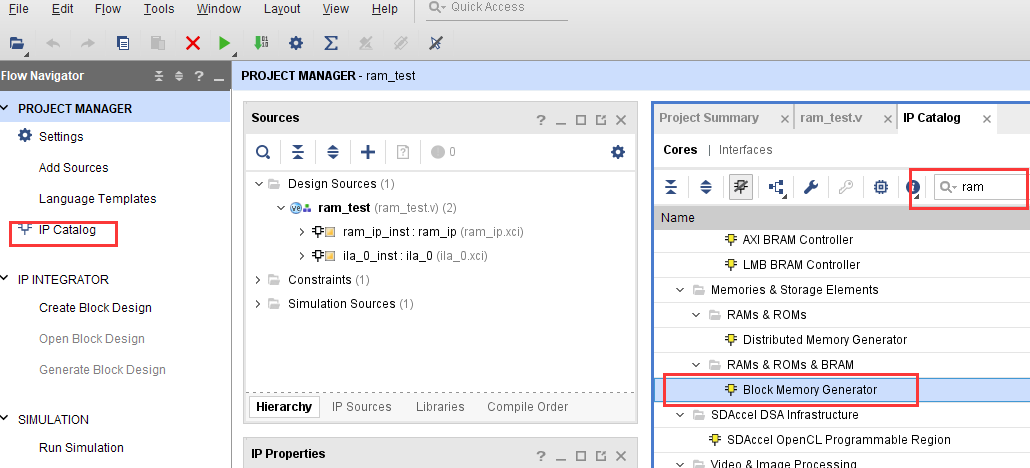
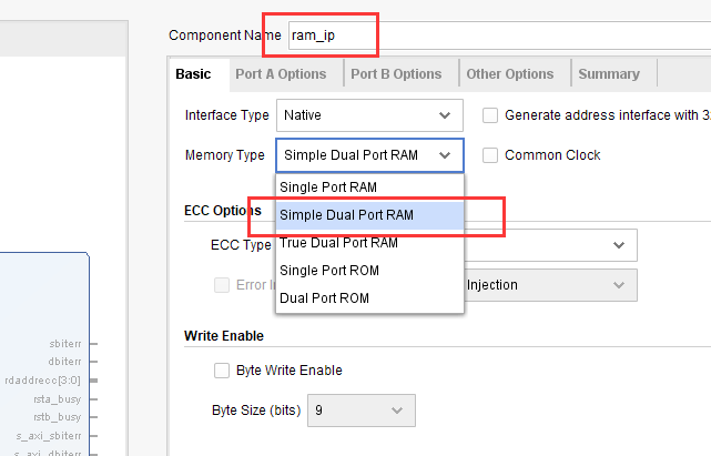
2. Change Component Name to ram_ip. Under the Basic tab, change Memory Type to Simple Dual Port RAM, that is, a simple dual-port RAM. Generally speaking, "Simple Dual Port RAM" is the most commonly used one, because it has two ports and the input and output signals are independent.
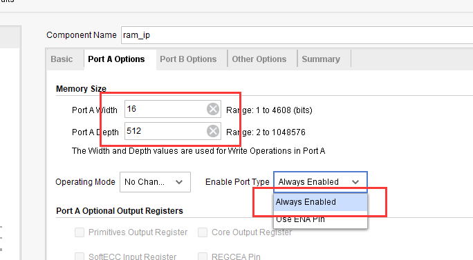
3. Switch to the Port A Options tab and change the RAM width Port A Width to 16, that is, the data width. Change the RAM depth Port A Depth to 512; depth means how many data items can be stored in the RAM. Change the enable pin Enable Port Type to Always Enable.
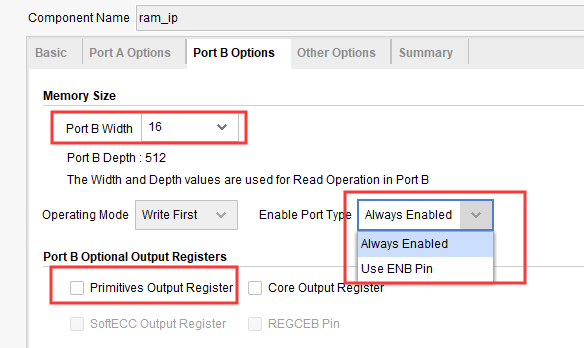
4. Switch to the Port B Options tab and change the RAM width Port B Width to 16, and change the enable pin Enable Port Type to Always Enable. Of course you can also use Use ENB Pin, which is equivalent to a read enable signal. Uncheck Primitives Output Register: its function is to add a register to the output data, which can effectively improve timing, but the read data will then lag the address by two cycles. In many cases this function is not enabled, keeping the data one cycle behind the address.
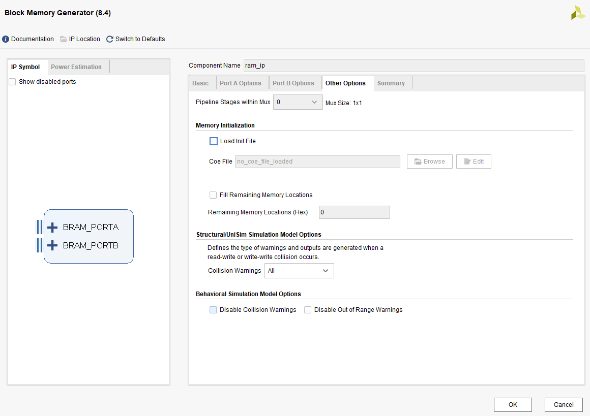
5. In the Other Options tab, unlike a ROM there is no need to initialise the RAM data here, because we can write it in the program, so the default configuration is sufficient; just click OK.
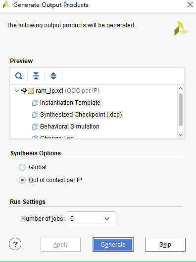
6. Click “Generate” to generate the RAM IP.
4.3 RAM Port Definitions and Timing
The ports of the Simple Dual Port RAM module are described as follows:
| Signal Name | Direction | Description |
| clka | in | Port A clock input |
| wea | in | Port A enable |
| addra | in | Port A address input |
| dina | in | Port A data input |
| clkb | in | Port B clock input |
| addrb | in | Port B address input |
| doutb | out | Port B data output |
Data is written to and read from the RAM on the rising edge of the clock. When writing data through port A, the wea signal must be driven high and the address and the data to be written must be provided at the same time. The figure below is the timing diagram of writing data into the RAM.
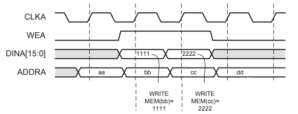
RAM write timing
Port B, however, cannot write data; it can only read data from the RAM, and providing the address is sufficient. Normally valid data can be captured in the next cycle.
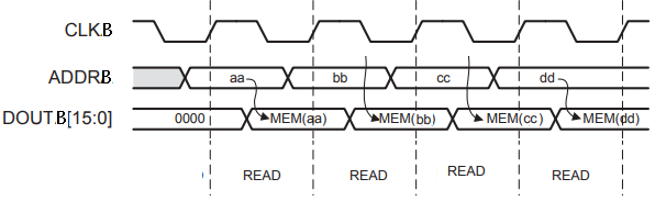
RAM read timing
4.4 Writing the Test Program
Next we write the test program for the RAM. To test the function of the RAM, we write a series of consecutive data to port A of the RAM, only once, and read it out from port B, using the logic analyser to view the data.
In order to see the data values read from the RAM in real time, we add the ila tool here to observe the data signal and the address signal of RAM PORTB. For how to generate ila, please refer to the chapter “The PL ‘Hello World’ LED Experiment”.
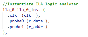
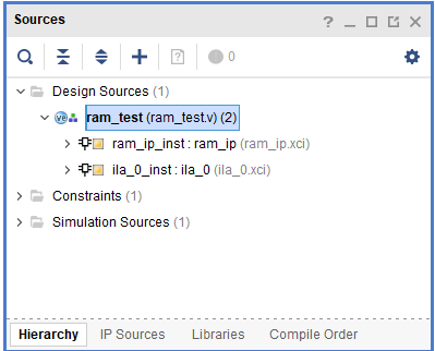
The program structure is as follows:
Pin binding
############## clock and reset define################## create_clock -period 20 [get_ports clk] set_property IOSTANDARD LVCMOS33 [get_ports {clk}] set_property PACKAGE_PIN U18 [get_ports {clk}] set_property IOSTANDARD LVCMOS33 [get_ports {rst_n}] set_property PACKAGE_PIN N15 [get_ports {rst_n}]
4.5 Simulation
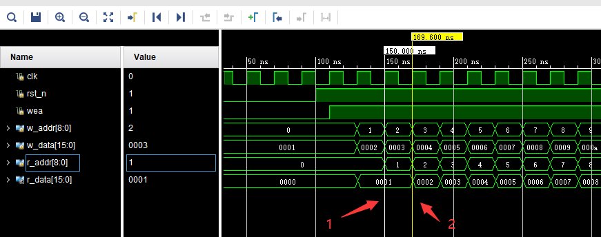
For the simulation method, refer to the chapter “The PL ‘Hello World’ LED Experiment”. The simulation results are as follows; from the figure you can see that the data written at address 1 is 0002, and in the next cycle, that is at moment 2, the valid data is read out.
4.6 Board Verification
Generate the bitstream and download the bit file to the FPGA. Next we use ila to observe whether the data read from the RAM is the data we initialised.
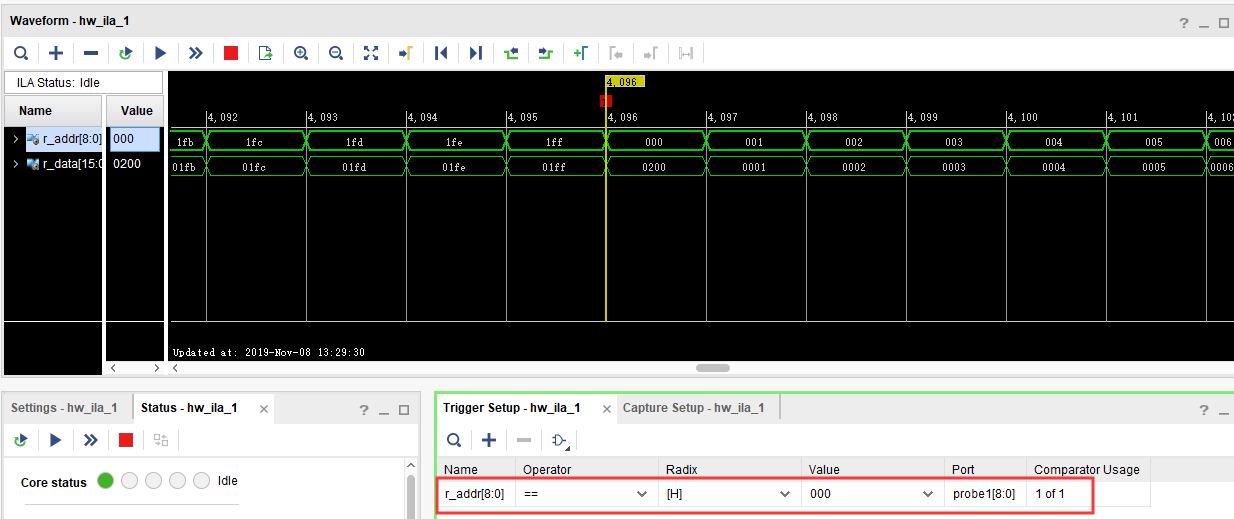
In the Waveform window, set the r_addr address to 0 as the trigger condition. We can see that r_addr keeps incrementing from 0 to 1ff, and as r_addr changes, r_data also changes. The data of r_data is exactly the 512 data items we wrote into the RAM. Note here that when a new address appears on r_addr, the corresponding data on r_data appears only after two clock cycles; the data appears two clock cycles later than the address, consistent with the simulation results.
Chapter 5 FPGA On-chip ROM Read/Write Test Experiment
The Vivado project for this experiment is “rom_test”.
The FPGA itself is of SRAM architecture, so the program disappears when the power is removed. How then can a ROM be implemented using an FPGA? We can use the RAM resources inside the FPGA to implement a ROM, but it is not a true ROM: every time power is applied, the initialised values are first written into the RAM. This experiment introduces how to use the ROM inside the FPGA and how a program reads data from that ROM.
5.1 Experiment Principle
Xilinx already provides a ROM IP core in VIVADO. We only need to instantiate a ROM through the IP core, then read the data stored in the ROM according to the ROM read timing. In the experiment, through the online logic analyser ila integrated in VIVADO, we can observe the ROM read timing and the data read from the ROM.
5.2 Program Design
5.2.1 Creating the ROM Initialisation File
Since it is a ROM, we must prepare the data for it in advance, and then when the FPGA actually runs we simply read the data pre-stored in the ROM. The on-chip ROM of a Xilinx FPGA supports initialisation data configuration. As shown in the figure below, we can create a file named rom_init.coe. Note that the extension must be “.coe”, while the name before it can of course be chosen freely.

The content format of the ROM initialisation file is very simple, as shown in the figure below. The first line defines the data format; 16 means that the data format of the ROM is hexadecimal. From line 3 to line 34 is the initialisation data of this 32×8-bit ROM. Each line of numbers is followed by a comma, and the last line ends with a semicolon.
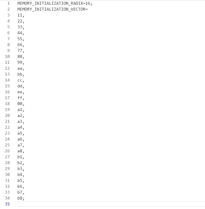
Once rom_init.coe has been written, save it. Next we begin to design and configure the ROM IP core.
5.2.2 Adding the ROM IP Core
Before adding the ROM IP, first create a project named rom_test, then add the ROM IP to the project, as follows:
1. Click IP Catalog as shown below, search for rom in the pane that pops up on the right, find Block Memory Generator and double-click it.
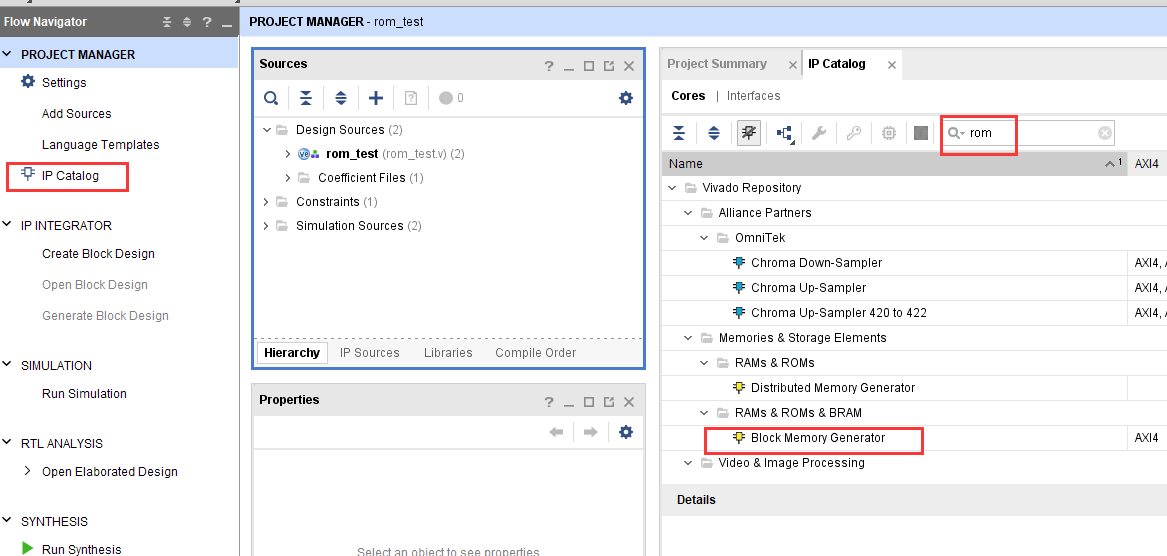
2. Change Component Name to rom_ip and, under the Basic tab, change Memory Type to Single Port ROM.
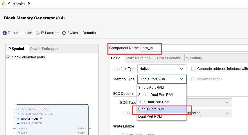
3. Switch to the Port A Options tab and change the ROM width Port A Width to 8, change the ROM depth Port A Depth to 32, change the enable pin Enable Port Type to Always, and uncheck Primitives Output Register.
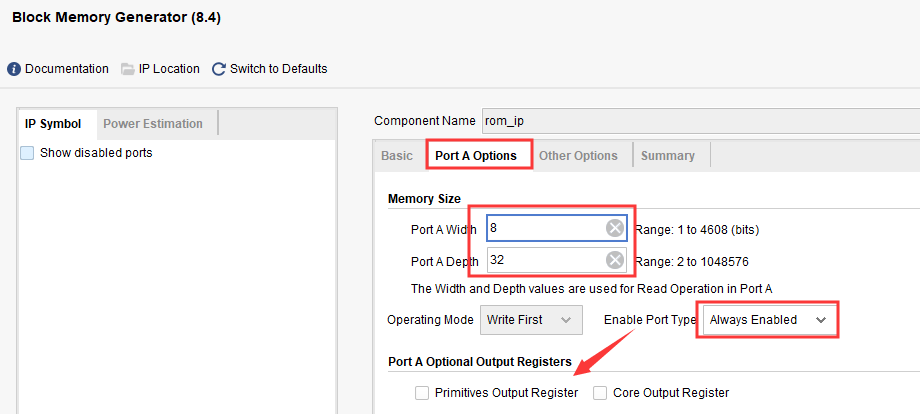
4. Switch to the Other Options tab, check Load Init File, click Browse, and select the .coe file prepared earlier.
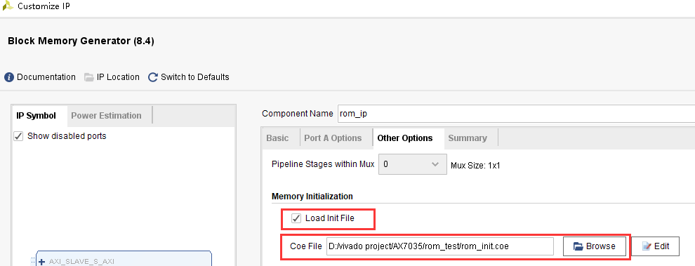
5. Click ok, then click Generate to generate the IP core.
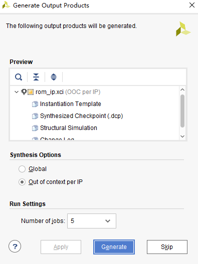
5.3 Writing the ROM Test Program
The ROM program design is very simple: in the program we only need to change the ROM address on every clock, and the ROM outputs the internal data stored at the current address. Instantiate ila to observe the changes of the address and the data.
5.4 Simulation
The simulation results are as follows and meet expectations. As with reading data from the RAM, the data lags the address by one cycle.
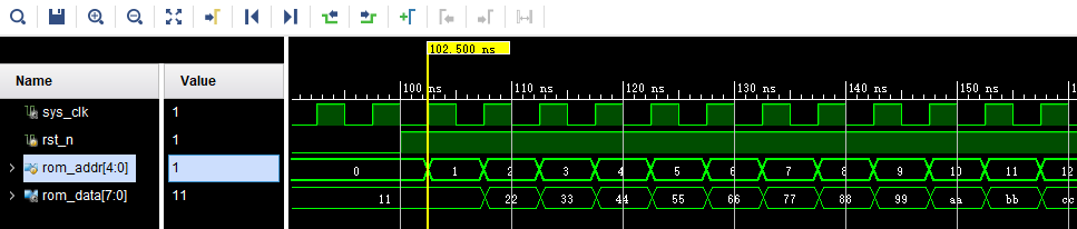
5.5 Board Verification
With address 0 as the trigger condition, you can see that the data read is consistent with the simulation.
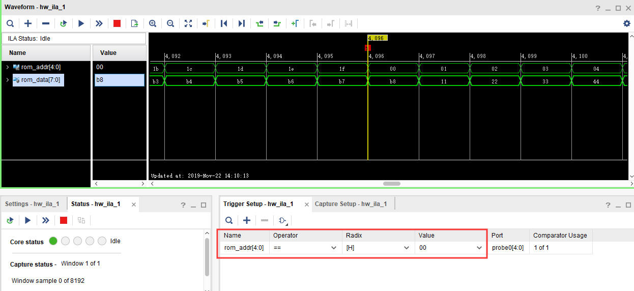
Chapter 6 FPGA On-chip FIFO Read/Write Test Experiment
The Vivado project for this experiment is “fifo_test”.
FIFO is a very important module in FPGA applications and is widely used for data caching, cross-clock-domain data processing and so on. Learning FIFO well is key to FPGA design, and being able to use FIFO flexibly is an essential skill for an FPGA engineer. This chapter mainly introduces read/write testing using the FIFO IP provided by XILINX.
6.1 Experiment Principle
FIFO: First in, First out means that the data that goes in first comes out first, and the data that goes in later comes out later. Xilinx already provides a FIFO IP core in VIVADO. We only need to instantiate a FIFO through the IP core, then write and read the data stored in the FIFO according to the FIFO read/write timing.
In fact a FIFO is based on RAM with many additional functions. The typical structure of a FIFO is as follows: it is mainly divided into a read part and a write part, plus status signals — the empty and full signals — and also a data count status signal. The biggest difference from RAM is that a FIFO has no address lines and cannot read data from random addresses. What does reading data at random mean? It means being able to read the data at any arbitrary address. A FIFO is different: it cannot perform random reads, and the advantage of this is that the address lines do not need to be controlled frequently.
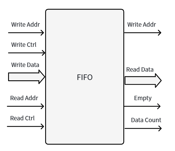
Although users cannot see the address lines, address operations still exist inside the FIFO, and they are used to control the read/write interface of the RAM. Its addresses during read and write operations are shown in the figure below, in which the depth value is the maximum number of data items that can be stored in one FIFO. In the initial state both the read and write addresses are 0. After one data item is written into the FIFO, the write address is incremented by 1; after one data item is read from the FIFO, the read address is incremented by 1. At this point the FIFO state is empty, because one data item was written and one data item was read out.
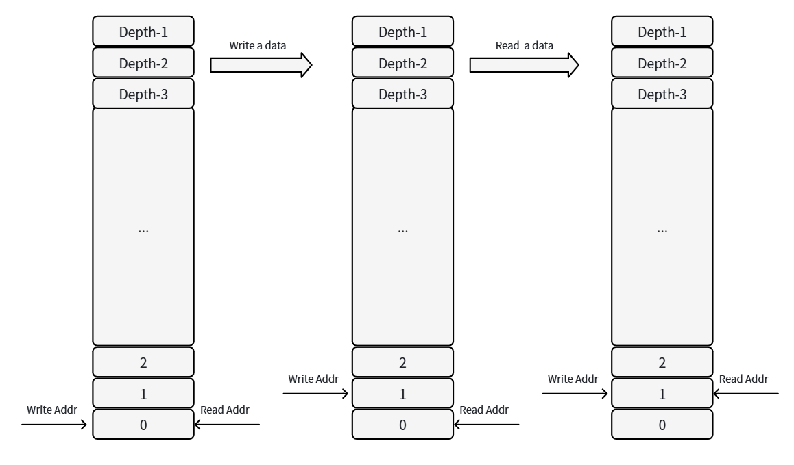
A FIFO can be imagined as a water tank: the write channel is filling it with water and the read channel is draining it. Suppose water is added and drained without interruption: if water is added faster than it is drained, the FIFO will eventually be full, and if water keeps being added when it is full it overflows; if water is drained faster than it is added, the FIFO will eventually be empty. So getting the moment and rate of filling and draining right, and keeping the tank always containing water, is a very demanding task. That is, you must judge the empty and full states and write or read data at the right moment.
According to the read and write clocks, FIFOs can be divided into synchronous FIFOs (the read and write clocks are the same) and asynchronous FIFOs (the read and write clocks are different). Synchronous FIFO control is relatively simple and is not covered here; this section mainly introduces the control of an asynchronous FIFO, in which the read clock is 75MHz and the write clock is 100MHz. In the experiment, through the online logic analyser ila integrated in VIVADO, we can observe the FIFO read/write timing and the data read from the FIFO.
6.2 Creating the Vivado Project
6.2.1 Adding the FIFO IP Core
Before adding the FIFO IP, first create a project named fifo_test, then add the FIFO IP to the project, as follows:
1. Click IP Catalog as shown below, search for fifo in the pane that pops up on the right, find FIFO Generator and double-click it.
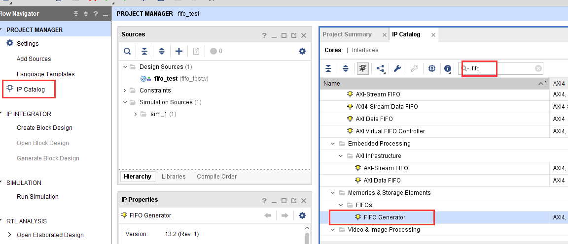
2. In the configuration page that pops up, you can choose whether the read and write clocks are separate or shared. Generally, when we use a FIFO to cache data, the clock speeds on the two sides are different, so independent clocks are the most commonly used. Here we select “Independent Clocks Block RAM”, then click “Next” to go to the next configuration page.
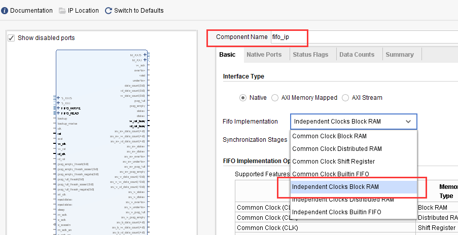
3. Switch to the Native Ports tab and select a data width of 16; select 512 for the FIFO depth (in actual use you can set it as needed). There are two Read Mode options: one is Standard FIFO, the FIFO we usually see, in which the data lags the read signal by one cycle; the other is First Word Fall Through, a data prefetch mode, abbreviated as FWFT mode. That is, the FIFO fetches one data item in advance, so that when the read signal is asserted the corresponding data is valid as well. We first perform the standard FIFO experiment.
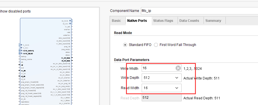
4. Switch to the Data Counts tab and enable Write Data Count (how much data has been written into the FIFO) and Read Data Count (how much data in the FIFO can be read), so that we can use these two values to see how much data there is inside the FIFO. Click OK and Generate to generate the FIFO IP.
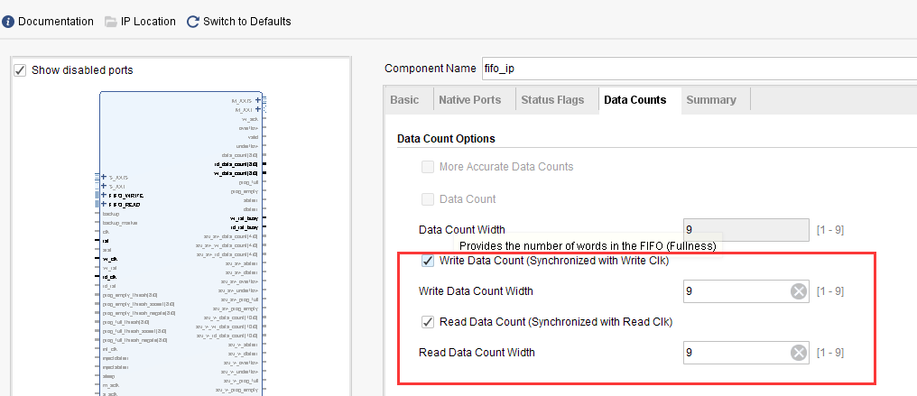
6.2.2 FIFO Port Definitions and Timing
| Signal Name | Direction | Description |
| rst | in | Reset signal, active high |
| wr_clk | in | Write clock input |
| rd_clk | in | Read clock input |
| din | in | Write data |
| wr_en | in | Write enable, active high |
| rd_en | in | Read enable, active high |
| dout | out | Read data |
| full | out | Full signal |
| empty | out | Empty signal |
| rd_data_count | out | Amount of readable data |
| wr_data_count | out | Amount of data written |
Data is written to and read from the FIFO on the rising edge of the clock. When the wr_en signal is high, data is written into the FIFO. When the almost_full signal is asserted, it means that only one more data item can be written into the FIFO; once that one data item has been written, the full signal is driven high. If wr_en is still asserted while full, that is, data continues to be written into the FIFO, the FIFO's overflow signal is asserted, indicating an overflow.
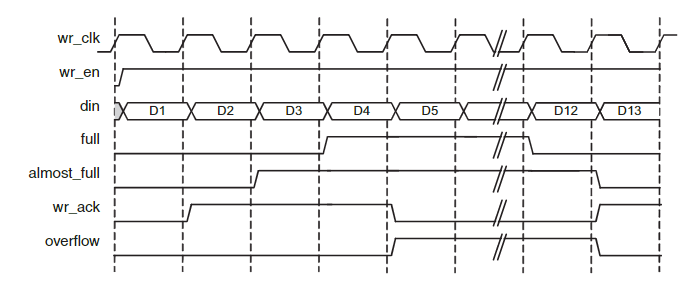
Standard FIFO write timing
When the rd_en signal is high, FIFO data is read, and the data is valid in the next cycle. valid is the data valid signal; almost_empty means there is still one data item to read. When one more data item is read, the empty signal is asserted; if reading continues, underflow is asserted, indicating an underflow, and the data read out at this time is invalid.
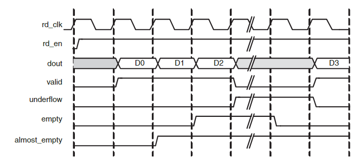
Standard FIFO read timing
From the timing diagram of reading data in FWFT mode it can be seen that when the rd_en signal is asserted, the valid data D0 is already prepared and valid on the data lines, and is not delayed by another cycle. This is the difference from a standard FIFO.
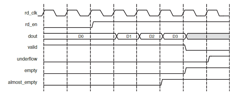
FWFT FIFO read timing
For detailed information about FIFO, refer to document pg057, which can be downloaded from the Xilinx website.
6.3 Writing the FIFO Test Program
We design according to an asynchronous FIFO, using a PLL to generate two clocks, 100MHz and 75MHz, which are used as the write clock and the read clock respectively; that is, the write clock frequency is higher than the read clock frequency.
In the program the lock signal of the PLL is used as the reset of the FIFO, and at the same time the 100MHz clock is assigned to the write clock and the 75MHz clock to the read clock.
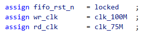
One point to note is that the FIFO uses the safety circuit by default. This function ensures that the input signals reaching the internal RAM are synchronised. With this enabled, after an asynchronous reset you must wait for 60 of the slowest clock cycles — in this experiment 60 cycles of the 75MHz clock — so for the 100MHz clock roughly (100/75)×60=80 cycles are needed.
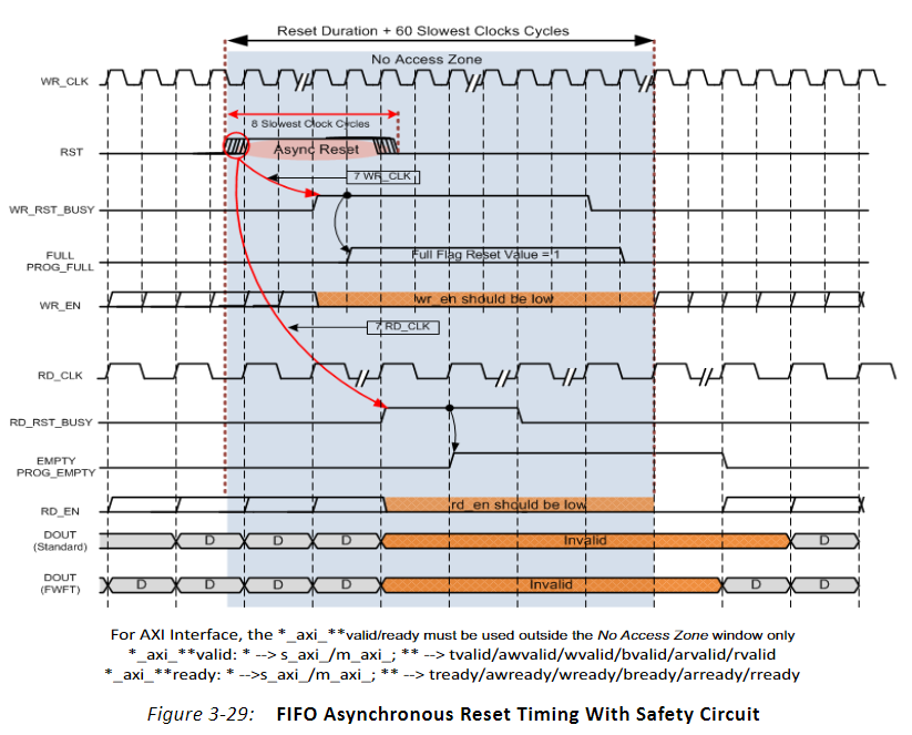
Therefore, in the write state machine, 80 cycles are waited before entering the write-FIFO state.
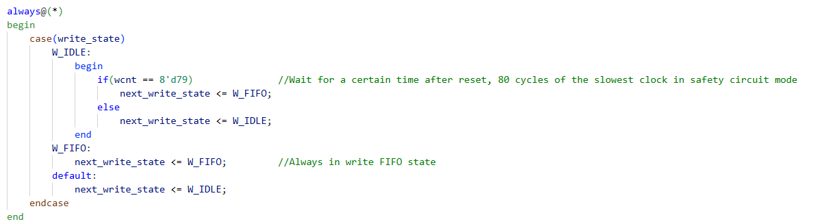
In the read state machine, 60 cycles are waited before entering the read state.
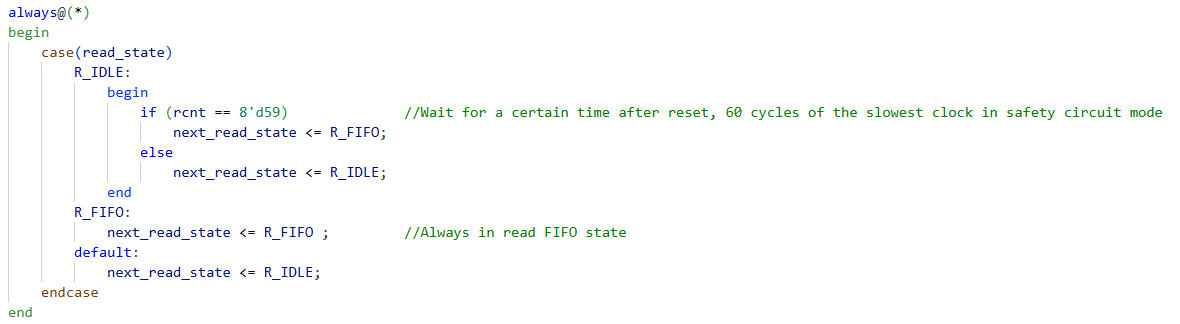
If the FIFO is not full, data continues to be written into the FIFO.

If the FIFO is not empty, data continues to be read from the FIFO.

Two logic analysers are instantiated, connected to the signals of the write channel and the read channel respectively.
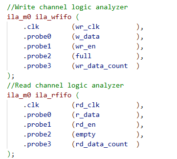
6.4 Simulation
The simulation results are as follows. After the write enable wr_en is asserted, data writing begins, with an initial value of 0001. A certain number of cycles are needed from the start of writing until empty is deasserted, because synchronisation is also performed internally. Once it is not empty, reading begins, and the read data lags rd_en by one cycle.
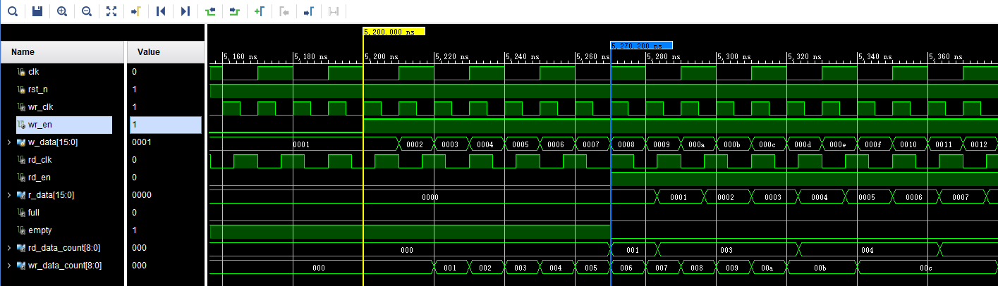
Later you can see that if the FIFO becomes full, according to the program design no more data is written into the FIFO once it is full, and wr_en is pulled low. Why does it become full? Because the write clock is faster than the read clock. If the write clock and the read clock are swapped, that is, if the read clock is faster, the FIFO will be read empty. You can try this for yourself.
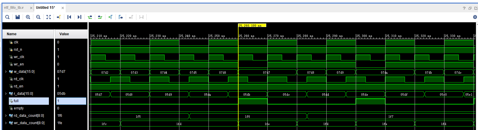
If the Read Mode of the FIFO is changed to First Word Fall Through
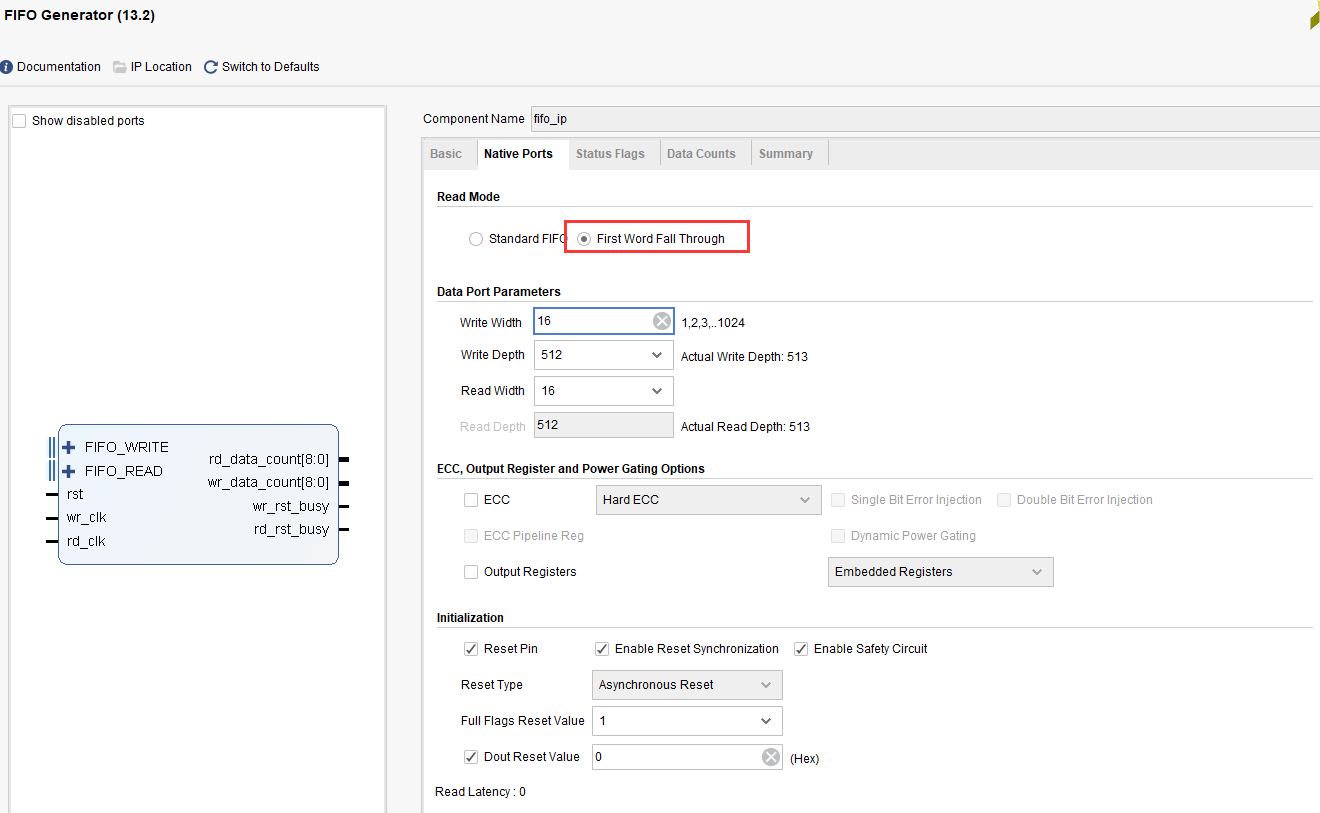
The simulation results are as follows; you can see that the data is valid when rd_en is asserted, with no one-cycle difference.
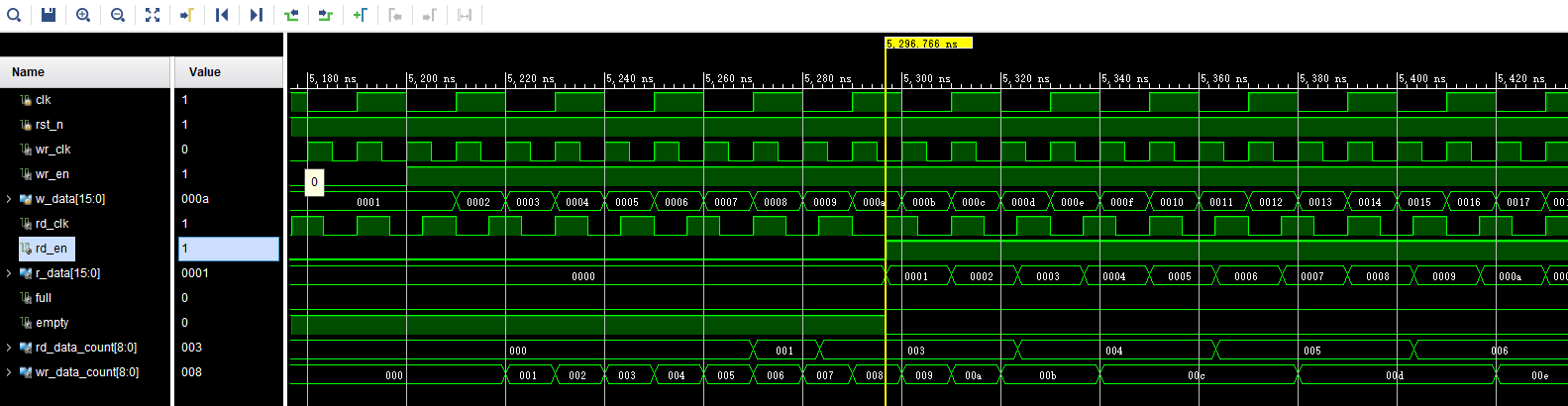
6.5 Board Verification
Generate the bit file and download it; two ila instances appear. First look at the write channel: you can see that when the full signal is high, wr_en is low and no more data is written into it.
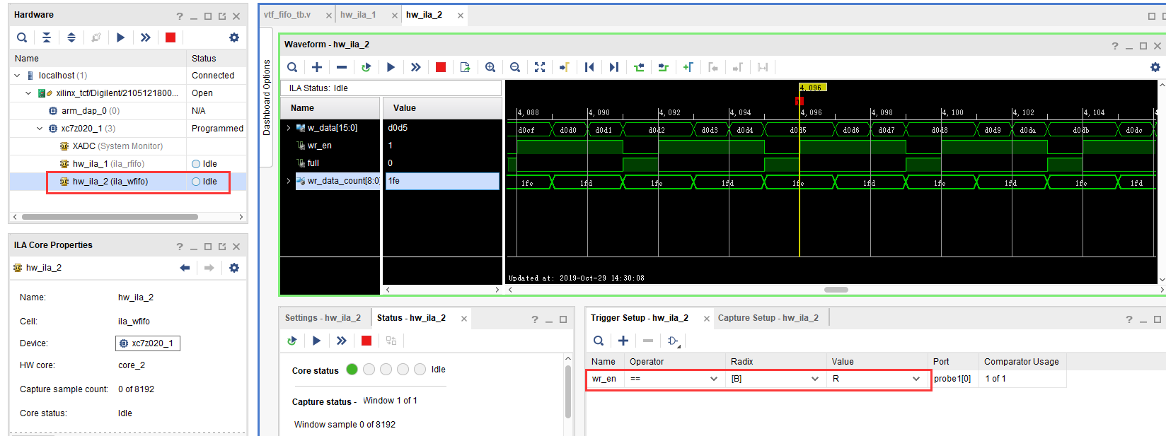
The read channel is also consistent with the simulation.
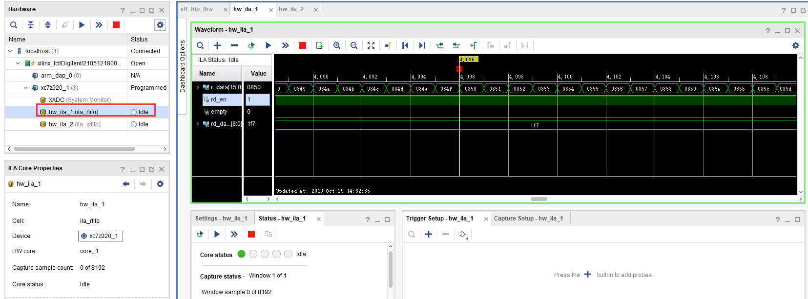
If the rising edge of rd_en is used as the trigger condition, click Run and then press reset, that is, the PL KEY1 we bound, the following result appears, consistent with the simulation: in standard FIFO mode the data lags rd_en by one cycle.
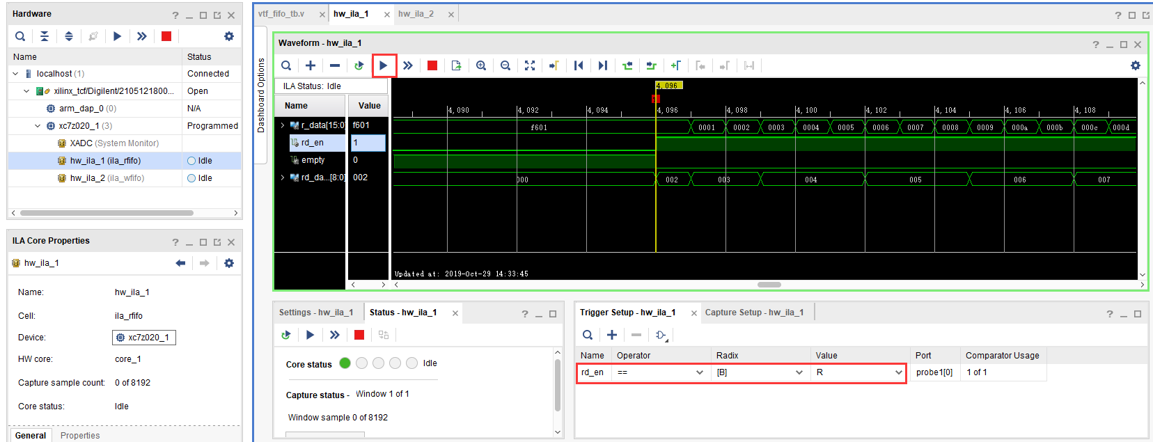
Chapter 7 Push-button Experiment in Vivado
The Vivado project for this experiment is “key_test”.
The push button is the most commonly used and simplest peripheral in FPGA design. In this chapter, through a button detection experiment, we check whether the button function of the development board works properly, and gain an understanding of the concrete relationship between the hardware description language and the FPGA, learning how to use Vivado RTL ANALYSIS.
7.1 Push-button Hardware Circuit
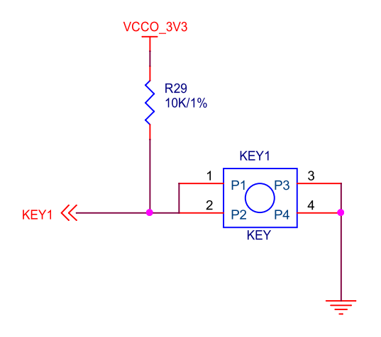
The push-button circuit of the development board
From the figure it can be seen that in this circuit the button is at a high level when released and at a low level when pressed.
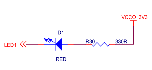
The LED circuit of the development board
As for the LED part, it is lit at a low level and off at a high level.
7.2 Program Design
This program is not designed to be very complex; through a simple hardware description language design it reveals the connection between the hardware description language and FPGA hardware. First we pass the button input through 2 groups of D flip-flops. A signal that has passed through a D flip-flop is latched on the rising edge of the flip-flop's clock input and then sent to the output.
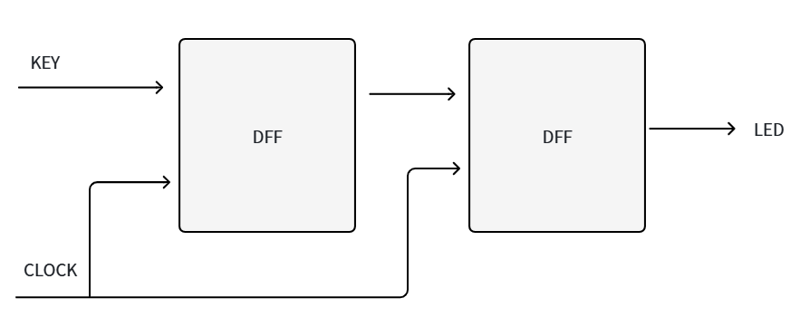
Before coding in a hardware description language we have already built the hardware; this is the normal development flow. Once you have the hardware design idea, the design can be completed either by drawing a schematic or by using Verilog HDL or VHDL; the tool is chosen according to the complexity of the design and your familiarity with a particular language.
7.3 Creating the Vivado Project
1. First create the button test project, add the Verilog test code, and complete the flow of compiling and assigning pins.
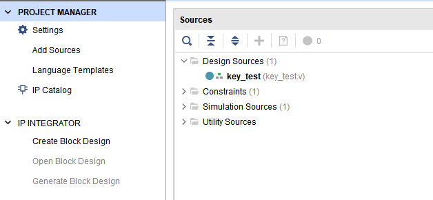
1
`timescale 1ns / 1ps
module key_test
(
    input clk, //system clock 50Mhz on board
    input key, //input four key signal,when the keydown,the value is 0
    output led //LED display ,when the siganl low,LED lighten
);

reg led_r; //define the first stage register , generate four D Flip-flop
reg led_r1; //define the second stage register ,generate four D Flip-flop

always@(posedge clk)
begin
    led_r <= key; //first stage latched data
end

always@(posedge clk)
begin
    led_r1 <= led_r; //second stage latched data
end

assign led = led_r1;

endmodule
2. We can use the RTL ANALYSIS tool to view the design.
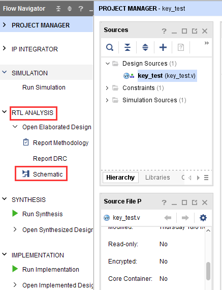
3. Analysing the RTL diagram, you can see that the first-stage D flip-flop is connected to the button input and the second stage takes its input directly from it, consistent with the intended design.
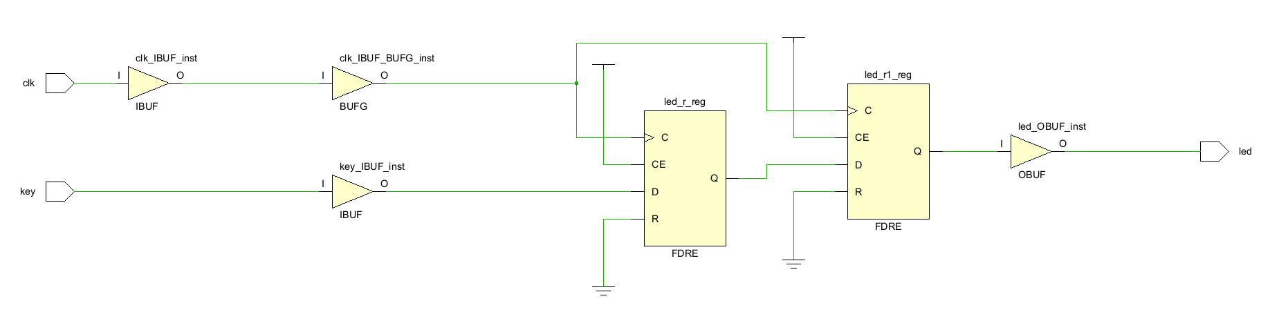
7.4 Board Verification
After the bit file is downloaded to the development board, the LED on the board is off, and the LED lights when the button is pressed.
Chapter 8 PWM Breathing LED Experiment
The Vivado project for this experiment is “pwm_led”.
This document mainly explains how to use PWM to control an LED and achieve the breathing-light effect.
8.1 Experiment Principle
As shown in the figure below, an N-bit counter is used whose maximum value can be expressed as 2 to the power N and whose minimum value is 0. The counter accumulates with “period” as the step value; after reaching the maximum value it overflows and enters the next accumulation period. When the counter value is greater than “duty”, the pulse output is high, otherwise it is low. In this way the pulse output with an adjustable duty cycle shown by the red line in the figure is produced, and at the same time “period” can adjust the pulse frequency; it can be understood as the step value of the counter.
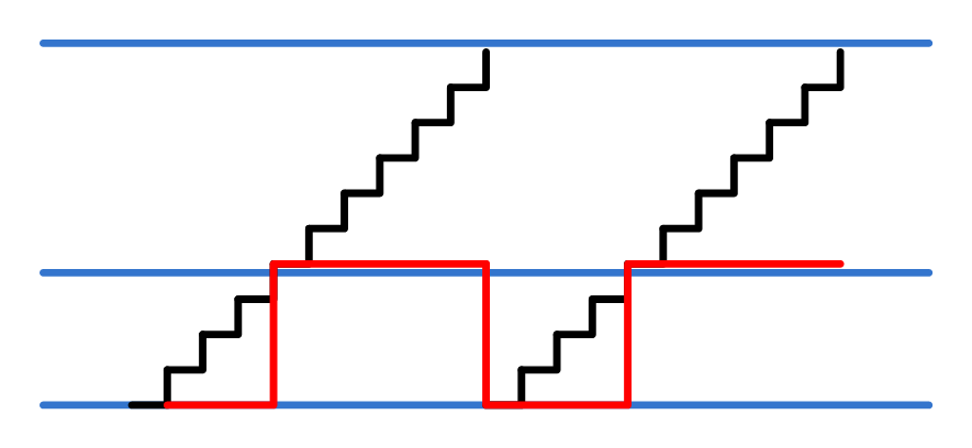
PWM pulse-width modulation diagram
When square waves with different pulse duty cycles are output and applied to the LED, the LED shows different brightness; by continuously adjusting the duty cycle of the square wave, the brightness of the LED is adjusted.
8.2 Experiment Design
The PWM module design is very simple and has already been covered in the principle above, so the principle is not repeated here.
| Signal Name | Direction | Description |
| clk | in | Clock input |
| rst | in | Asynchronous reset input, active high |
| period | in | PWM pulse period (frequency) control. period = PWM output frequency * (2 to the power N) / system clock frequency. Obviously, the larger N is, the higher the frequency accuracy. |
| duty | in | Duty cycle control. Duty cycle = duty / (2 to the power N) * 100% |
Ports of the PWM module (ax_pwm)
1
`timescale 1ns / 1ps
module ax_pwm
#(
parameter N = 16 //pwm bit width
)
(
    input clk,
    input rst,
    input[N - 1:0]period, //pwm step value
    input[N - 1:0]duty, //duty value
    output pwm_out //pwm output
);

reg[N - 1:0] period_r; //period register
reg[N - 1:0] duty_r; //duty register
reg[N - 1:0] period_cnt; //period counter
reg pwm_r;

assign pwm_out = pwm_r;

always@(posedge clk or posedge rst)
begin
    if(rst==1)
    begin
        period_r <= { N {1'b0} };
        duty_r <= { N {1'b0} };
    end
    else
    begin
        period_r <= period;
        duty_r <= duty;
    end
end

//period counter, step is period value
always@(posedge clk or posedge rst)
begin
    if(rst==1)
        period_cnt <= { N {1'b0} };
    else
        period_cnt <= period_cnt + period_r;
    end

always@(posedge clk or posedge rst)
begin
    if(rst==1)
    begin
        pwm_r <= 1'b0;
    end
    else
    begin
        if(period_cnt >= duty_r) //if period counter is bigger or equals to duty value, then set pwm value to high
            pwm_r <= 1'b1;
        else
            pwm_r <= 1'b0;
    end
end

endmodule
So how is the breathing-light effect achieved? We know that the breathing-light effect is the process in which the light goes from dim to continuously brighter and then from bright to continuously dimmer, and the brightness is adjusted by the duty cycle. We therefore mainly control the duty cycle, that is, control the value of duty.
In the test code below, the value of period is set so that the PWM frequency is 200Hz. The PWM_PLUS state increments the duty value; if it reaches the maximum value, pwm_flag is set to 1 and the duty value starts to be decreased, and once it has decreased to the minimum value the duty value starts to increase again, repeating continuously. The PWM_GAP state is the adjustment interval, whose duration is 100us.
1
`timescale 1ns / 1ps
module pwm_test(
                 input 		clk,		//50MHz
                 input 		rst_n,		//low active
	             output 	led			//high-off, low-on
                );

localparam CLK_FREQ = 50 ; 				//50MHz
localparam US_COUNT = CLK_FREQ ; 		//1 us counter
localparam MS_COUNT = CLK_FREQ*1000 ; 	//1 ms counter

localparam DUTY_STEP	  = 32'd100000 ;	//duty step
localparam DUTY_MIN_VALUE = 32'h6fffffff ;	//duty minimum value
localparam DUTY_MAX_VALUE = 32'hffffffff ;	//duty maximum value

localparam IDLE    		= 0;	//IDLE state
localparam PWM_PLUS  	= 1;    //PWM duty plus state
localparam PWM_MINUS  	= 2;    //PWM duty minus state
localparam PWM_GAP  	= 3;    //PWM duty adjustment gap

wire 		pwm_out;	//pwm output
reg[31:0] 	period;		//pwm step value
reg[31:0] 	duty;		//duty value
reg			pwm_flag ;	//duty value plus and minus flag, 0: plus; 1: minus

reg[3:0] 	state;
reg[31:0] 	timer;		//duty adjustment counter

assign led = ~pwm_out ; //led low active

always@(posedge clk or negedge rst_n)
begin
    if(rst_n == 1'b0)
    begin
    	period 		<= 32'd0;
    	timer 		<= 32'd0;
    	duty 		<= 32'd0;
    	pwm_flag 	<= 1'b0 ;
    	state 		<= IDLE;
    end
    else
    case(state)
    	IDLE:
    	begin
    		period 		<= 32'd17179;   //The pwm step value, pwm 200Hz(period = 200*2^32/50000000)
    		state  		<= PWM_PLUS;
    		duty   		<= DUTY_MIN_VALUE;
    	end
    	PWM_PLUS :
    	begin
    		if (duty > DUTY_MAX_VALUE - DUTY_STEP)	//if duty is bigger than DUTY MAX VALUE minus DUTY_STEP , begin to minus duty value
    		begin
    			pwm_flag 	<= 1'b1 ;
    			duty   		<= duty - DUTY_STEP ;
    		end
    		else
    		begin
    			pwm_flag 	<= 1'b0 ;
    			duty   		<= duty + DUTY_STEP ;
    		end

    		state  		<= PWM_GAP ;
    	end
    	PWM_MINUS :
    	begin
    		if (duty < DUTY_MIN_VALUE + DUTY_STEP)	//if duty is little than DUTY MIN VALUE plus duty step, begin to add duty value
    		begin
    			pwm_flag 	<= 1'b0 ;
    			duty   		<= duty + DUTY_STEP ;
    		end
    		else
    		begin
    			pwm_flag 	<= 1'b1 ;
    			duty   		<= duty - DUTY_STEP ;
    		end
    		state  		<= PWM_GAP ;
    	end
    	PWM_GAP:
    	begin
    		if(timer >= US_COUNT*100)      //adjustment gap is 100us
    		begin
    			if (pwm_flag)
    				state <= PWM_MINUS ;
    			else
    				state <= PWM_PLUS ;

    			timer <= 32'd0;
    		end
    		else
    		begin
    			timer <= timer + 32'd1;
    		end
    	end
    	default:
    	begin
    		state <= IDLE;
    	end
    endcase
end

//Instantiate pwm module
ax_pwm
#(
  .N(32)
 )
ax_pwm_m0(
    .clk      (clk),
    .rst      (~rst_n),
    .period   (period),
    .duty     (duty),
    .pwm_out  (pwm_out)
    );

endmodule
8.3 Download Verification
Generate the bitstream and download the bit file; you can see the PL LED1 producing a breathing-light effect. PWM is a fairly commonly used module, for example for fan speed control, motor speed control and so on.
Chapter 9 HDMI Output Experiment
The Vivado project for this experiment is “hdmi_output_test”.
We introduced the LED blinking experiment above only in order to understand the basic Vivado development flow. The experiment in this chapter is somewhat more complex than the LED blinking experiment: it produces colour bars on an HDMI output, and it is also the foundation for our later study of displays and video processing. The experiment does not yet involve the PS system; from the design of the experiment it can be seen that good FPGA fundamentals are required to make very good use of the ZYNQ chip.
9.1 Hardware Introduction
The development board does not use an HDMI encoder chip; instead, the FPGA's 3.3V differential IOs are connected directly to the HDMI connector, and the FPGA performs the 24-bit RGB encoding and outputs TMDS differential signals.
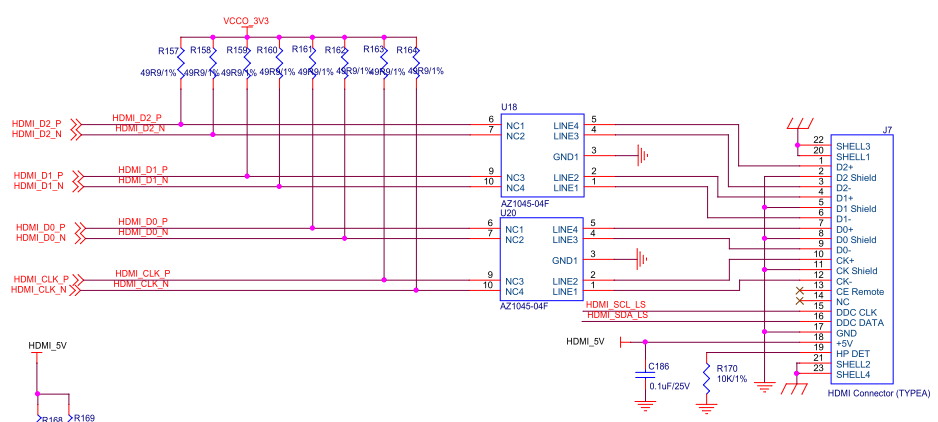
9.1.1 TMDS Principle
HDMI uses the same transmission principle as DVI — TMDS (Transition Minimized Differential signal).
The TMDS transmission system is divided into two parts: the transmitter and the receiver. The TMDS transmitter receives the 24-bit parallel data representing the RGB signals from the HDMI interface (TMDS encodes the three primary colours of each pixel separately at 8 bits, that is, the R signal has 8 bits, the G signal has 8 bits and the B signal has 8 bits), then encodes this data and performs parallel-to-serial conversion, and then distributes the data representing the 3 RGB signals to independent transmission channels for transmission. The receiver receives the serial signals from the transmitter, decodes them and performs serial-to-parallel conversion, and then sends them to the control end of the display. At the same time it also receives the clock signal in order to achieve synchronisation.
The principle of TMDS
Each TMDS link includes 3 data channels for transmitting the RGB signals and 1 channel for transmitting the clock signal. Each data channel uses an encoding algorithm to convert 8-bit video and audio data into 10-bit data with minimised transitions and DC balance. This makes the transmission and recovery of data more reliable. The transition-minimised differential signal converts the original 8-bit signal data into 10 bits through logical algorithms such as XOR and XNOR: the first 8 bits are obtained by processing the original signal, the 9th bit indicates the method of processing, and the 10th bit is used for DC balance.
Generally speaking, the encoding format transmitted over HDMI must contain video data, control data and data packets (data packets contain audio data and additional information data such as error correction codes). Each TMDS channel contains, when transmitting, a 2-bit control datum, 8-bit video data or a 4-bit data packet. The HDMI information transmission process can be divided into three stages: the video data period, the control data period and the data island period, corresponding respectively to the three data types above.
The techniques used in TMDS are described below:
- Transition minimisation
8-bit data is encoded and DC-balanced to obtain 10-bit minimised data. This appears to add redundant bits and to place higher bandwidth requirements on the transmission link, but in fact the 10-bit data obtained by this algorithm has enhanced reliability when transmitted over longer coaxial cables. The figure below is an example showing the encoding and parallel-to-serial conversion of 8-bit parallel RED data.
Step 1: send the 8-bit parallel RED data to the TMDS transmitter.
Step 2: parallel-to-serial conversion.
Step 3: perform the transition minimisation processing and add the 9th bit, that is, the encoding process. The 9th bit of data is called the encoding bit.
- DC balance
DC-balanced means ensuring during encoding that the DC offset in the channel is zero. The method is to add the 10th bit of data after the original 9 bits of data, so that the transmitted data tends towards DC balance, which reduces the electromagnetic interference that the signal causes on the transmission line and improves the reliability of signal transmission.
- Differential signal
TMDS differential transmission is a technique that uses the voltage difference between 2 pins to transmit a signal. The value of the transmitted data (“0” or “1”) is determined by the polarity and magnitude of the voltage between the two pins. That is, 2 wires are used to transmit the signal: the original signal is transmitted on one wire and the signal opposite to the original signal on the other wire. In this way the receiver can suppress electromagnetic interference by subtracting the signal on one wire from the signal on the other, thereby obtaining the correct signal.
As shown in the figure below:
In addition, there is a Display Data Channel (DDC), a signal line used to read the Extended Display Identification Data (EDID) that describes the display capabilities of the receiving monitor, such as its definition. Sending and receiving devices equipped with HDCP (High-bandwidth Digital Content Protection) also use the DDC line to authenticate the cipher keys.
9.1.2 Video Timing Standard
The HDMI display scan starts from a point at the upper left corner of the screen and scans point by point from left to right. After each line has been scanned, the electron beam returns to the starting position of the next line at the left of the screen, during which the CRT blanks the electron beam; at the end of each line, synchronisation is performed with the horizontal sync signal. When all lines have been scanned, a frame is formed; field synchronisation is performed with the vertical sync signal, the scan returns to the upper left of the screen, vertical blanking is performed at the same time, and the next frame begins.
The time taken to complete the scan of one line is called the horizontal scan time, and its reciprocal is called the line frequency; the time taken to complete the scan of one frame (the whole screen) is called the vertical scan time, and its reciprocal is called the field frequency, that is, the frequency at which the screen is refreshed, commonly 60Hz, 75Hz and so on. The field frequency of a standard display is 60Hz.
Clock frequency: taking 1024x768@59.94Hz (60Hz) as an example, each field corresponds to 806 line periods, of which 768 are display lines. Each display line includes 1344 pixel clocks, of which 1024 are the active display area. From this it can be seen that the required pixel clock frequency is 806134460, approximately 65MHz.
Video timing
In VGA scanning the basic element is the line scan, and multiple lines make up one frame. The figure below shows the timing of one line, in which the “Active” Video is the active pixels of one video line; for most resolution timings the Top/Left Border and the Bottom/Right Border are both 0. “Blanking” is the synchronisation time of one line, and the “Blanking” time plus the “Active” Video time is the time of one line. “Blanking” is further divided into three segments: “Front Porch”, “Sync” and “Back Porch”.

Line sync timing
The following are the timing parameters for 720p
1280x720@60Hz timing parameters
9.2 Creating the Vivado Project
This experiment implements HDMI output display: Verilog programming drives the HDMI output and displays a test pattern of colour bars on an HDMI monitor. The HDMI output display module is implemented as 3 modules: the clock module video_pll, the colour bar generation module color_bar and the VGA-to-DVI module rgb2dvi. The implemented logic block diagram is as follows:
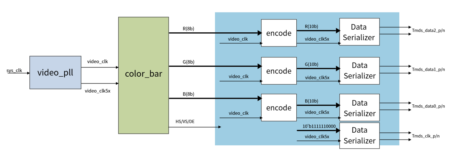
9.2.1 Adding the HDMI Encoder IP Core
1. Create a new project named “hdmi_output_test”.
Many people are fairly familiar with VGA data, which is RGB data, whereas HDMI is a TMDS differential signal. RGB data is relatively easy to handle in an FPGA, so what we need to do is convert the RGB data into HDMI TMDS differential signals; for this we use the RGB to DVI IP (both DVI and HDMI are TMDS signals).
2. Copy the repo folder (this folder can be found in the example project provided) into the project directory. This folder contains the HDMI encoder IP, which is provided by another vendor.
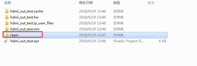
3. Click “IP Catalog”. By default these IP are all provided by Xilinx; now we want to add third-party IP, or IP made by ourselves.
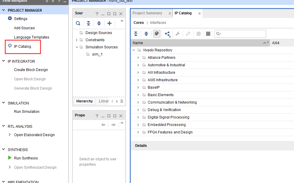
4. Right-click “Add Repository...”.
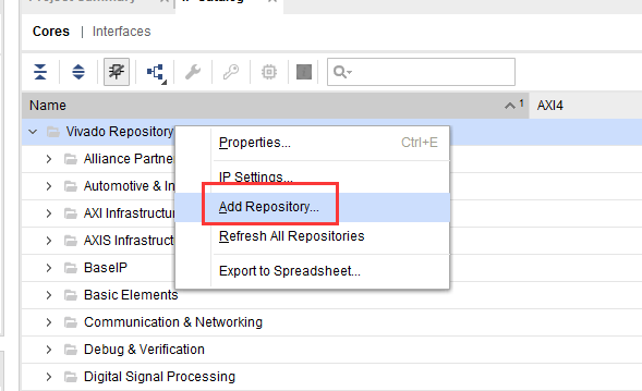
5. For the path, select the repo folder just copied.
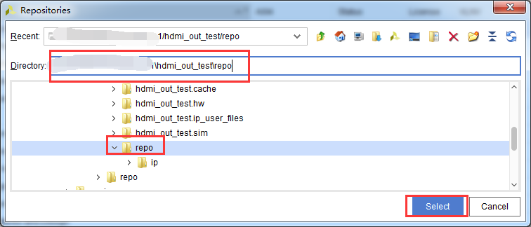
6. If the IP is added successfully, a message tells how many IP have been added.
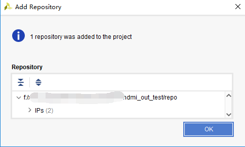
7. Find “RGB to DVI Video Encoder(Source)” and double-click it.
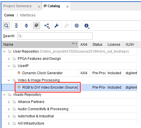
8. In the window that pops up below, leave the “Component Name” unchanged and leave the other parameters unchanged too; click “OK”.
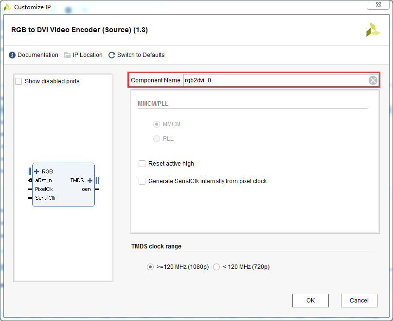
9. A “Generate Output Products” window pops up, in which “Number of jobs” refers to the number of threads; the higher it is, the faster.
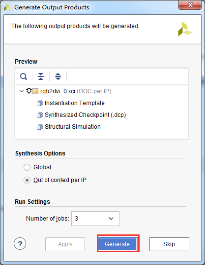
10. You can see one named rgb2dvi_0.
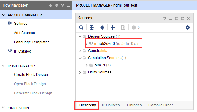
9.2.2 Adding the Pixel Clock PLL Module
In order to drive the HDMI encoder, a pixel clock and a clock at 5 times the pixel clock must be provided; the 5× pixel clock is used for 10:1 serialisation.
1. Search for the keyword “clock” in the “IP Catalog” window and double-click “Clocking Wizard”.
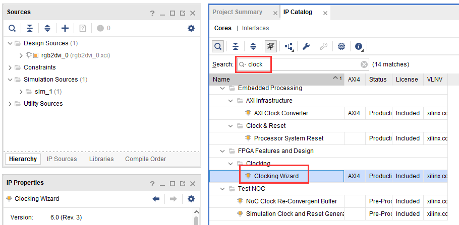
2. This time give the component a name: enter “video_clock” in “Component Name” and 50 for “clk_in1”; 50MHz matches the oscillator frequency on the PL side of the development board.
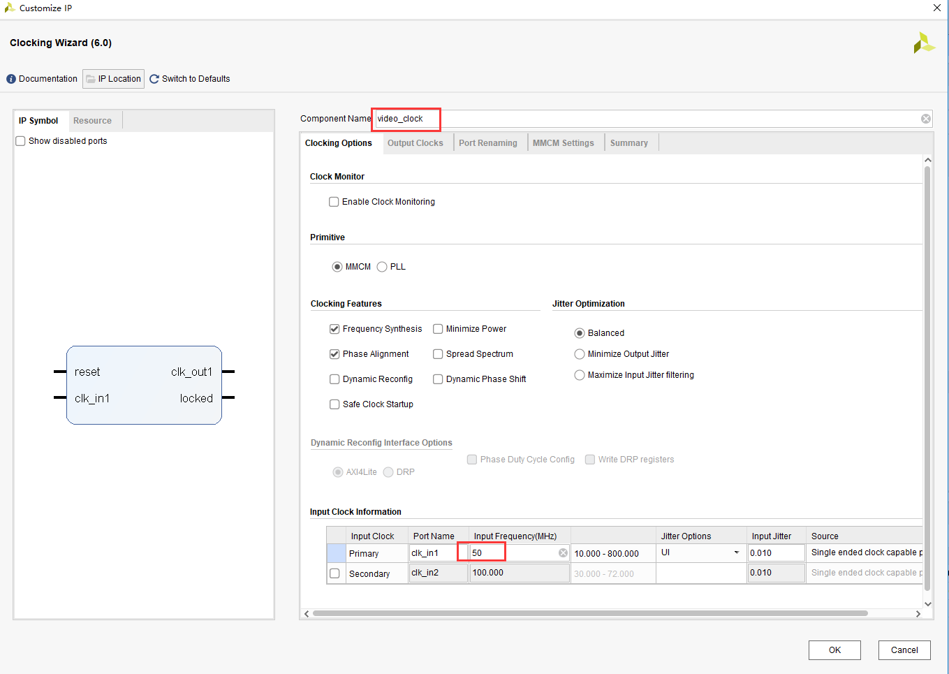
3. The output clock “clk_out1” is used as the video pixel clock; enter 74.25 here, which is the pixel clock for the 1280x720@60 resolution. Each resolution has a different pixel clock, and you need a very good understanding of video standards in order to know the pixel clock for each video resolution. “clk_out2” is used for encoder serialisation, at 5 times the pixel clock; enter 371.25 here, then click “OK” to generate the IP.
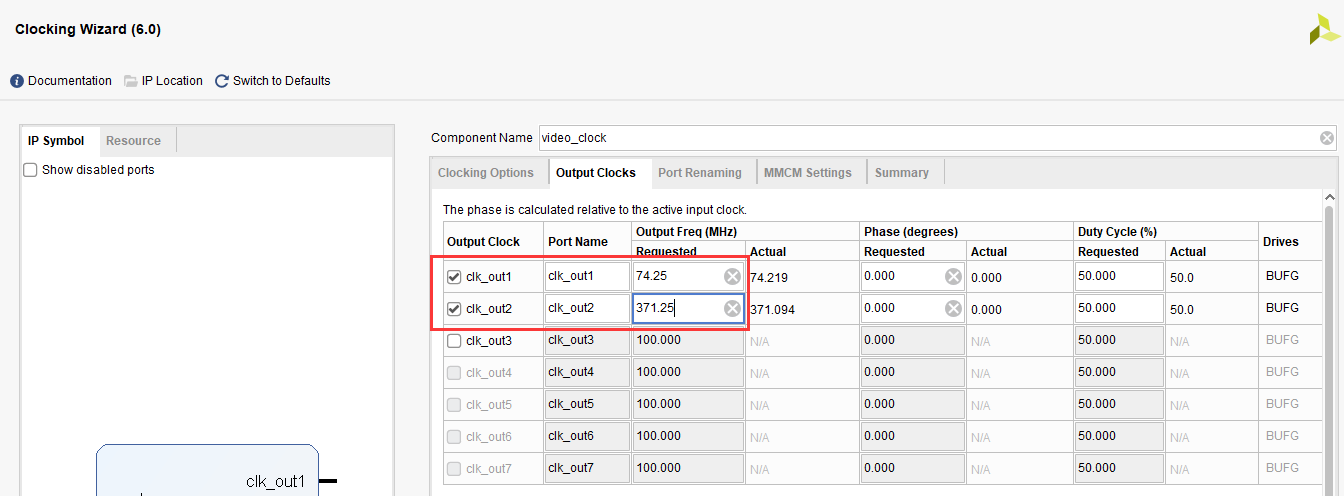
9.2.3 Adding the Colour Bar Generation Module
4. The colour bar generation module is a piece of Verilog code used to generate the video timing and the 8 horizontal colour bars; you can copy the existing code from the example provided. Parameters for different resolutions are defined in the color_bar file for users to use.
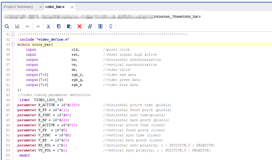
Add the video_define file, in which the macros for 1280x720 are defined

9.2.4 Adding the Top-level Module
5. The top module instantiates the colour bar generation module, the HDMI encoding module and the pixel clock generation module; for the code refer to the example project provided.
9.3 Adding the XDC Constraint File
Add the xdc constraint file to the project; the clock and HDMI-related pins have been added in the constraint file.
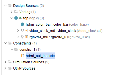
9.4 Download and Debug
Save the project, compile it and generate the bit file, and connect the HDMI interface to an HDMI monitor. Note that 1280x720@60Hz is used here, so please make sure that your monitor supports this resolution.
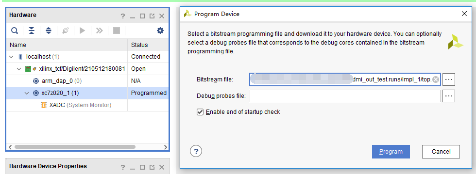
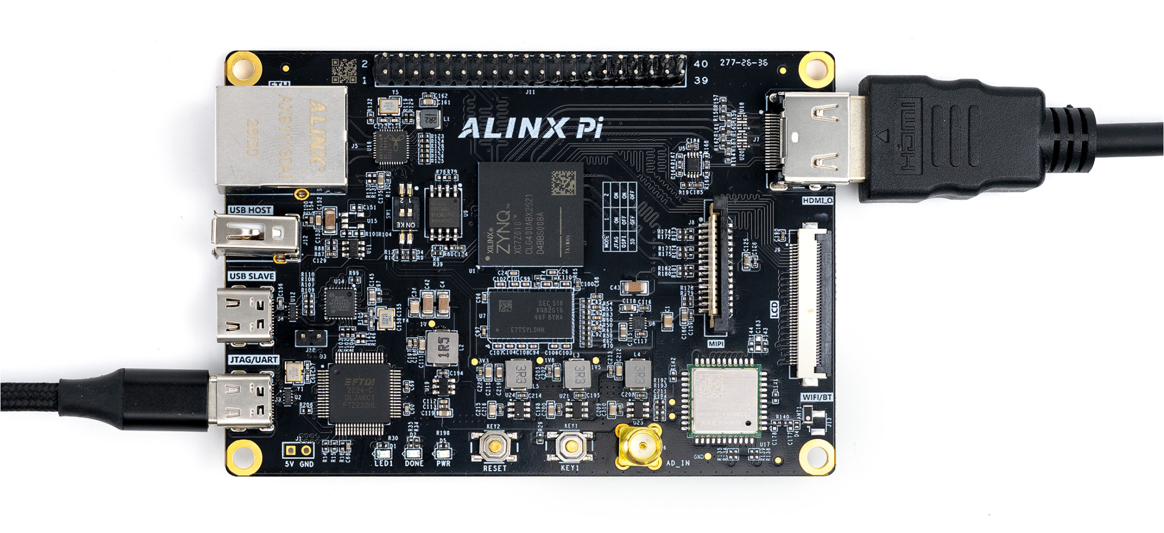
Hardware connection diagram
After downloading, the monitor displays the following image
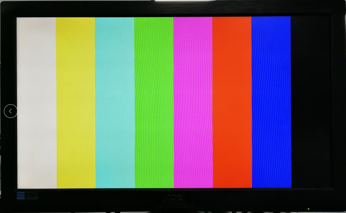
9.5 Experiment Summary
This experiment gives a first contact with video display and involves video knowledge, which is not the focus of ZYNQ study; ZYNQ is widely used in the video processing field and requires learners to have good basic knowledge. The experiment uses only the PL to drive the HDMI chip, giving a first look at how third-party custom IP is used; later we will learn how to define our own IP.
Chapter 10 HDMI Character Display Experiment
The Vivado project for this experiment is “hdmi_char”.
The HDMI output experiment explained the HDMI display principle and display method. This experiment introduces how to implement character display with an FPGA, and through this experiment you will gain a deeper understanding of the HDMI display method.
10.1 Experiment Principle
In the experiment a character conversion tool converts characters into a hexadecimal coe file, which is stored in a single-port ROM IP core; the converted data is then read out of the ROM and displayed on the HDMI output.
10.2 Program Design
The character display example adds an osd_display module on the basis of the HDMI display. The “osd_display” module is used to read the converted character information stored in the Rom IP core and display it in a specified area. The block diagram of the program is as follows:
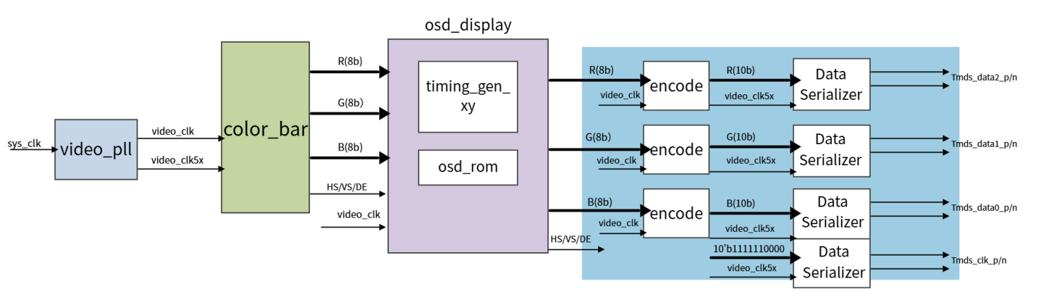
1. In the “timing_gen_xy” module, two counters “x_cnt” and “y_cnt” are defined according to the HDMI timing standard, and these two counters generate the “x” coordinate and the “y” coordinate of the HDMI display. In the program “vs_edge” and “de_falling” represent the field sync start signal and the data valid end signal respectively. The principle is shown in the figure below:
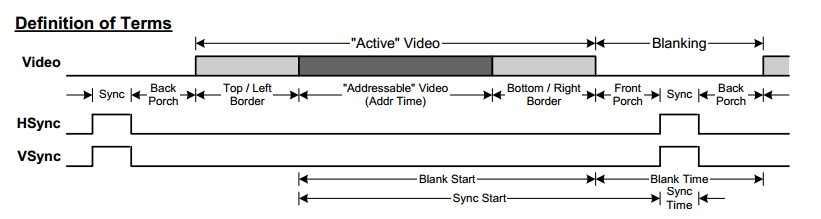
2.
| Signal Name | Direction | Description |
| rst_n | in | Asynchronous reset input, active low |
| clk | in | External clock input |
| i_hs | in | Horizontal sync signal |
| i_vs | in | Vertical sync signal |
| i_de | in | Data valid signal |
| i_data | in | color_bar data |
| o_hs | out | Output horizontal sync signal |
| o_vs | out | Output vertical sync signal |
| o_de | out | Output data valid signal |
| o_data | out | Output data |
| x | out | Generated X coordinate |
| y | out | Generated Y coordinate |
Ports of the timing_gen_xy module
3. Below we introduce the ROM IP used to store the text information. First a .coe file that can be recognised by a XILINX FPGA must be generated.
First find the “FPGA character dot-matrix extraction” tool in the project folder.

Double-click the .exe file to open the tool, and enter the characters to be displayed in the “character input” box of the extraction tool; the font and character height can be selected as you wish. When the settings are done, click the “Convert” button; the size of the converted character dot matrix can be seen at the lower left of the interface, and the width and height of the dot matrix are needed in the program.
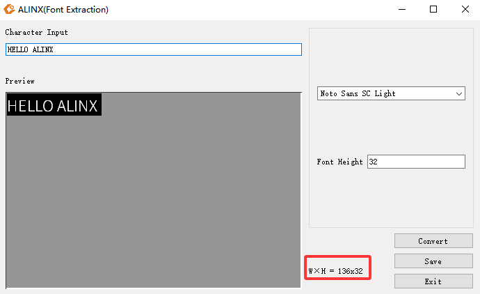
The width and height of the dot matrix here are 136x32, and they must be consistent with the definitions in the osd_display program:

Click the “Save” button. Note that under the save type you should select Xilinx (*.coe), then click the “Save” button.
Open the generated .coe file and you can see the following:
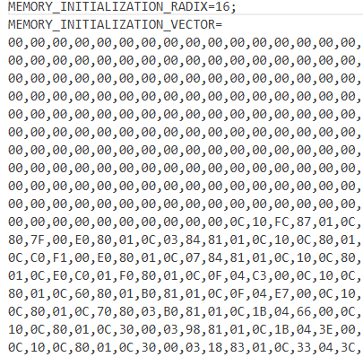
The procedure for instantiating a single-port Rom IP core has already been introduced in the earlier use of ROM; set it to Single Port ROM.
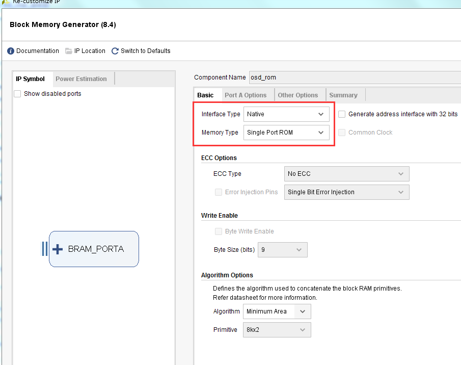
In the PortA Options tab, make the settings as follows:
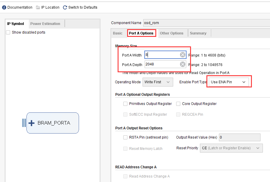
Add the osd.coe file as shown below (find the coe file generated earlier), then click the “OK” button when done:
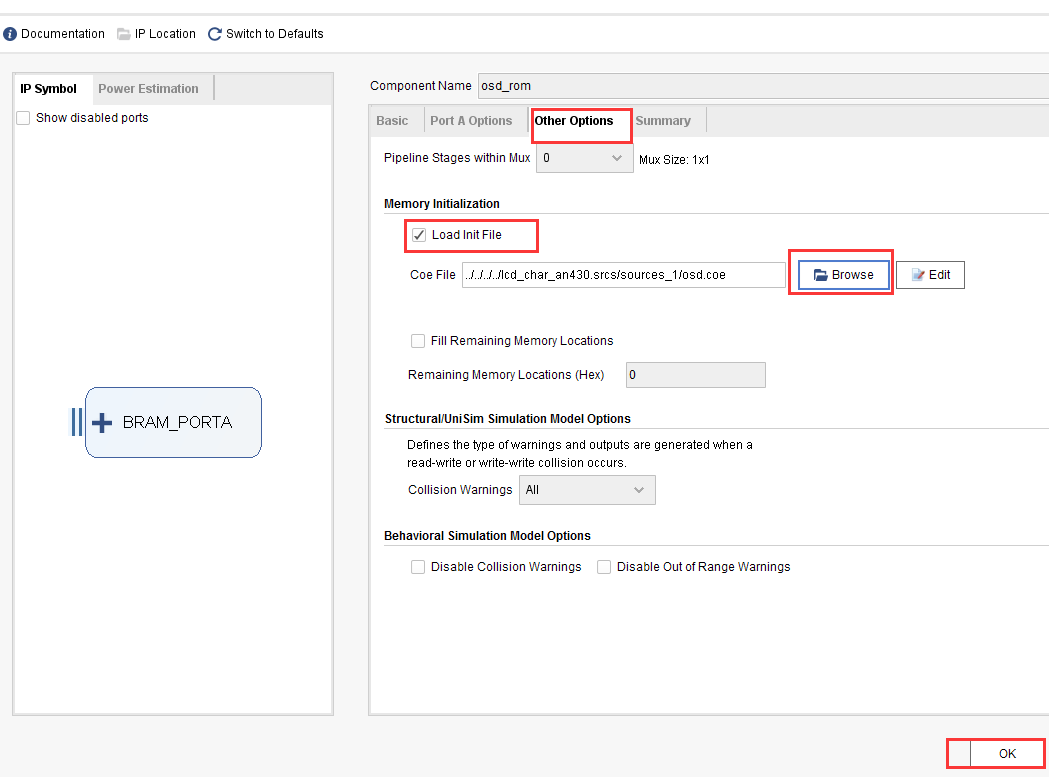
4. The osd_display module contains the timing_gen_xy module and the osd_rom module. As for the character data stored in osd_rom, if the data is 1 the OSD area displays the foreground red from the ROM (displaying the ALINX text), and if the data is 0 the OSD area displays the background colour (colour bars).
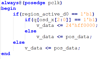
An area valid signal is set, that is, the character is displayed within this area. The starting coordinate is set to (9, 9), and the area size can be set according to the area set in the character generation tool.

Many people may not understand the ROM read address part: why is it [15:3], that is, one data item is read out only every eight clock cycles? This is because one dot of a character represents only 1 bit, whereas the data width stored in the ROM is 8 bits, so eight cycles are needed to fetch one data item, and the value of each bit is compared in order to convert one dot of the character into one pixel in the image.
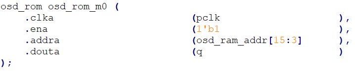
| Signal Name | Direction | Description |
| rst_n | in | Asynchronous reset input, active low |
| pclk | in | External clock input |
| i_hs | in | Horizontal sync signal |
| i_vs | in | Vertical sync signal |
| i_de | in | Data valid signal |
| i_data | in | color_bar data |
| o_hs | out | Output horizontal sync signal |
| o_vs | out | Output vertical sync signal |
| o_de | out | Output data valid signal |
| o_data | out | Output data |
Ports of the osd_display module
10.3 Experiment Results
Connect the development board and the monitor, referring to the "HDMI Output Experiment" tutorial for the connection method. Note that the various connectors on the development board must not be hot-plugged while powered. Download the experiment program and you can see the monitor displaying characters with colour bars as the background. As an HDMI output device, the development board can only be displayed through an HDMI display device; do not attempt to display through the HDMI port of a laptop, because a laptop is also an output device.
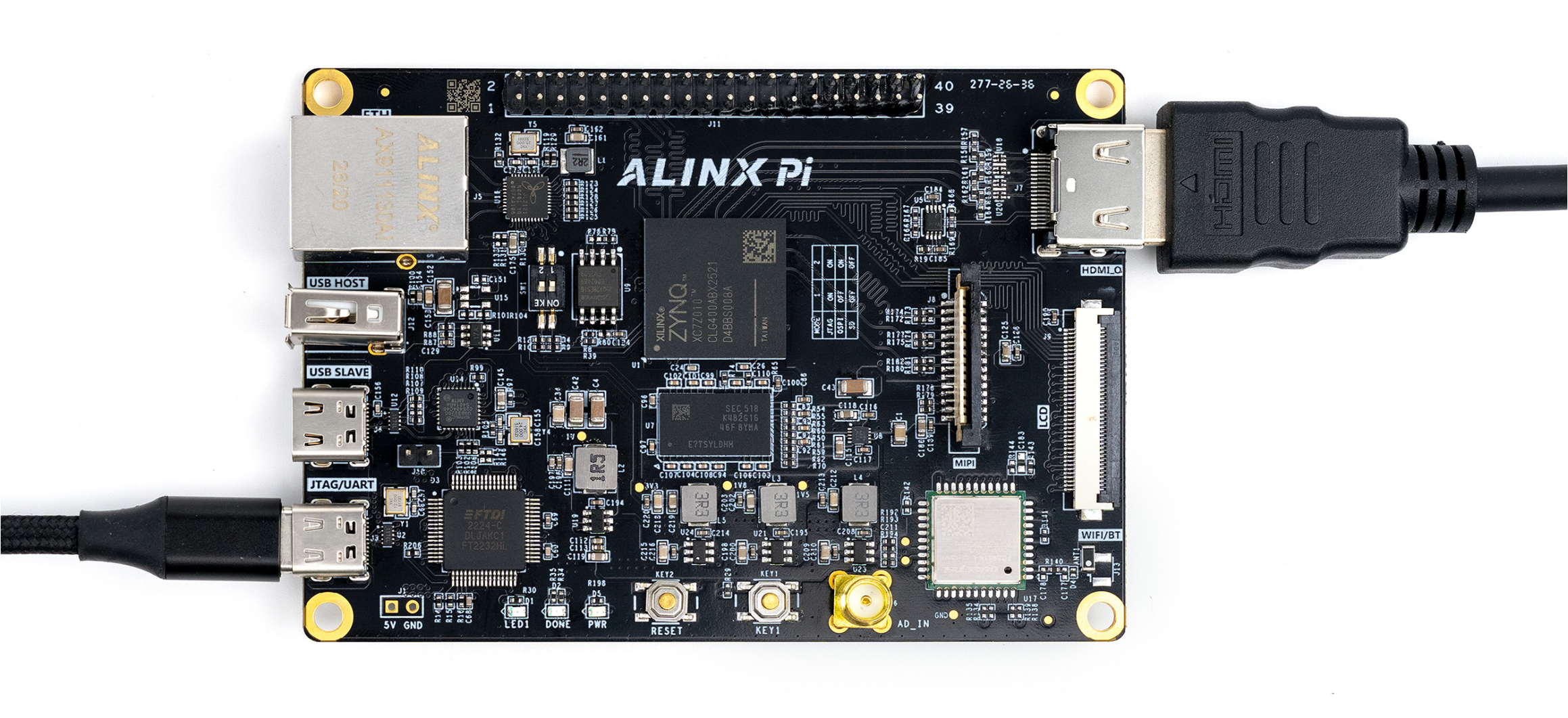
Hardware connection diagram

By default the character is displayed at the coordinate (9, 9). In addition, users can modify the judgment conditions for pos_y and pos_x below to display the character anywhere on the screen:

Chapter 11 LCD Display Experiment
The Vivado project for this experiment is “lcd_test”.
Building on the HDMI output experiment, this chapter introduces display on a 4.3-inch LCD panel.
11.1 Program Design
The experiment in this chapter is actually very simple. The biggest difference from the HDMI display is that the rgb-to-dvi module is not needed and the output can simply be RGB. The file structure is as follows, with the rgb2dvi module removed.
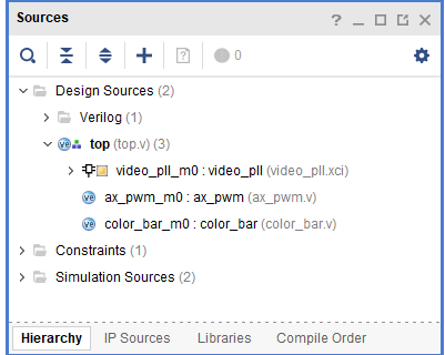
Also, because the resolution of the LCD panel is 800x480, the macro definitions in video_define.v must be modified.
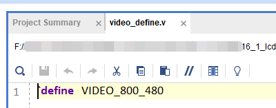
At the same time the output clock frequency of the PLL is changed to 33MHz, which is the pixel clock for 800x480.
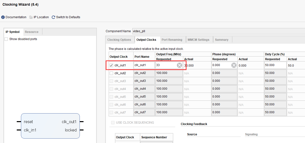
In addition, ax_pwm is instantiated in top.v to adjust the brightness of the LCD panel, set to 200Hz with a 30% duty cycle.
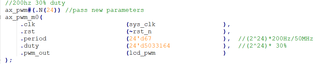
11.2 Experiment Results
Connect the LCD panel and download the program, and you will see the colour bars displayed.
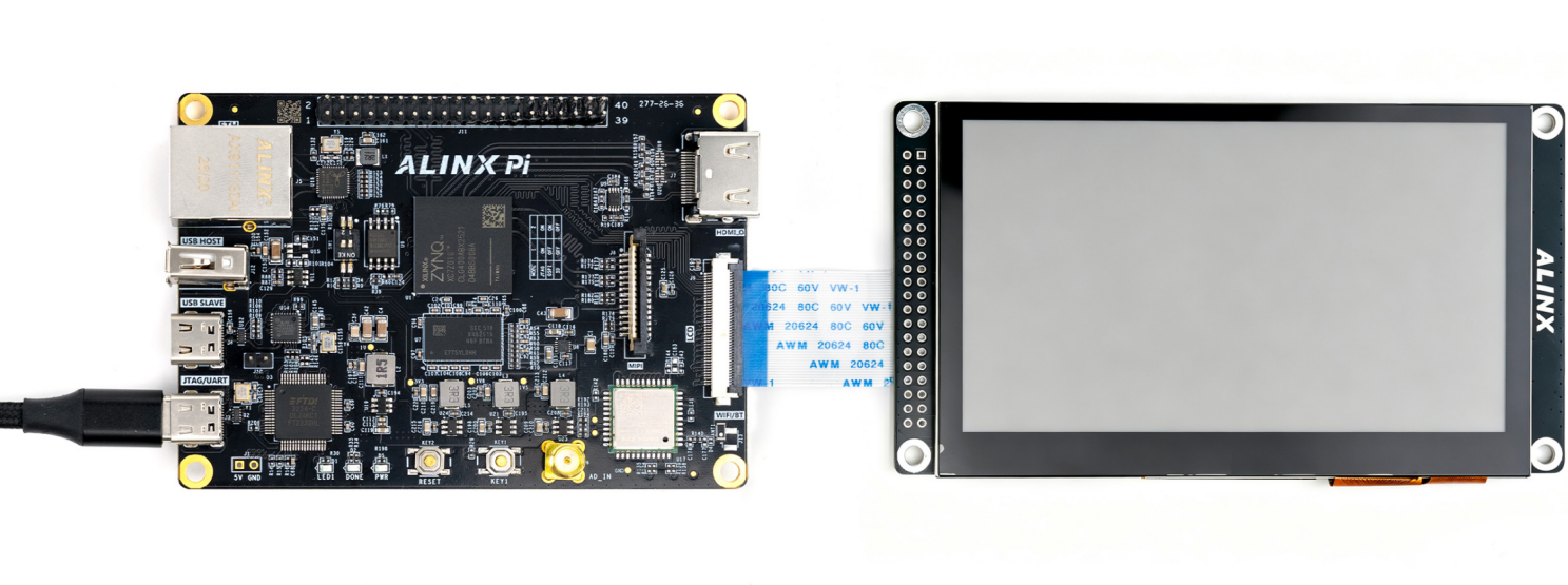
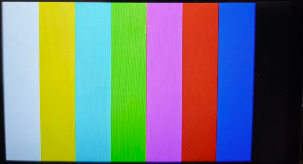
Connection of the ribbon cable on the back of the LCD panel
A character display example is also provided:
Character display
Chapter 12 XADC Waveform Acquisition and Display Experiment
The Vivado project for this experiment is “xadc_hdmi_test”.
This experiment practises using the XADC to acquire data and display it in the form of a waveform on the HDMI output, so that we can observe waveforms in a more intuitive way. It is the prototype of a digital oscilloscope.
12.1 Experiment Principle
The XADC is a two-channel 12-bit ADC with a 1M sampling rate, together with on-chip sensors. It can acquire the FPGA temperature, voltages and external module inputs; the acquired voltage range is 0-1V.
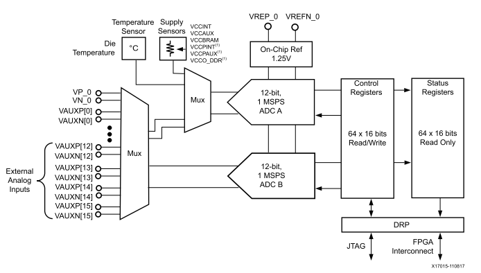
On the development board, a voltage divider circuit provides a 0-10V voltage acquisition range
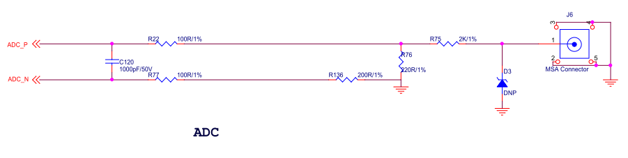
and it is connected to the VP and VN pins
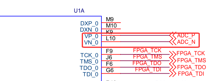
12.2 Program Design
The display part of this experiment is based on the earlier HDMI colour bar display experiment, with grid lines and a waveform superimposed on the colour bars. The block diagram of the whole project is as follows:
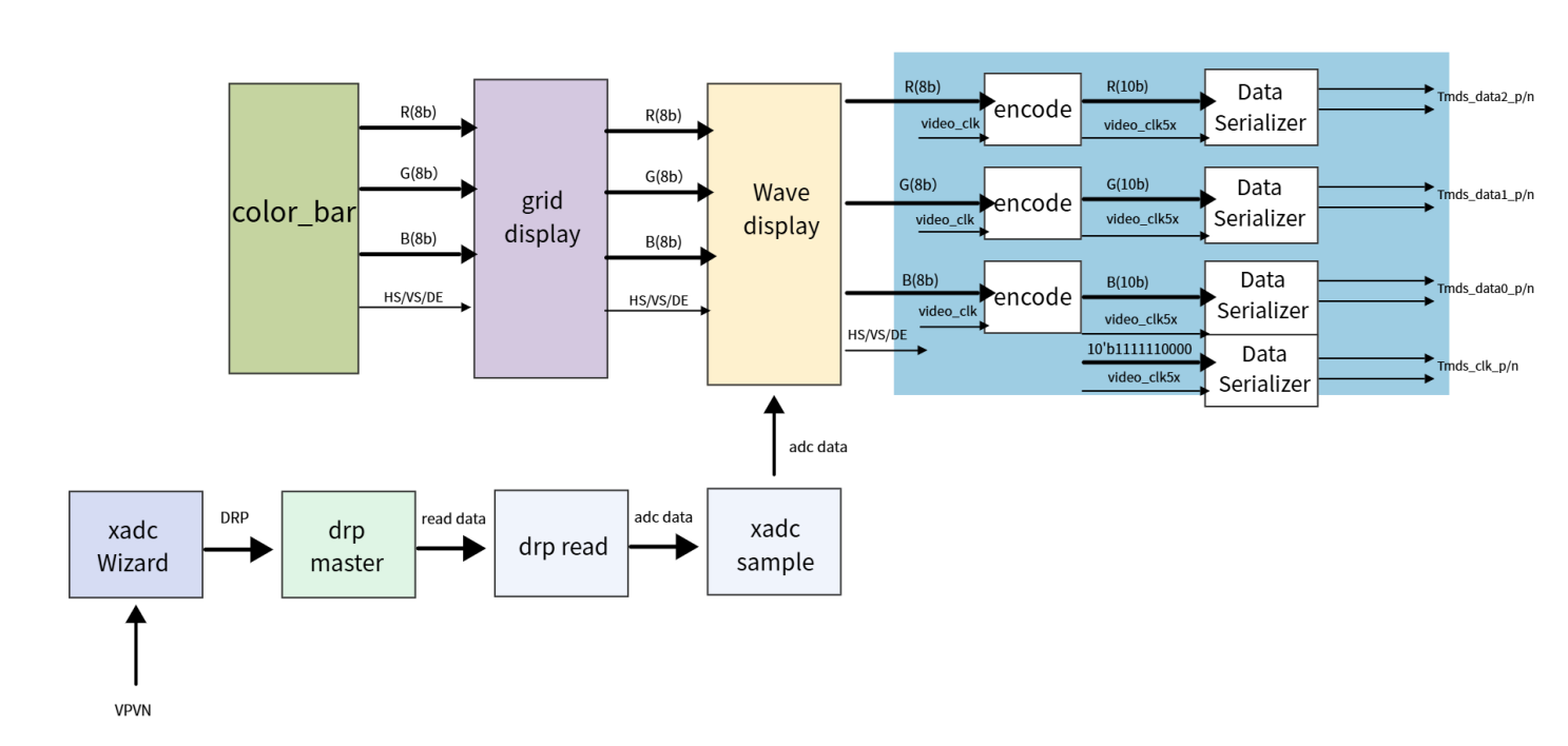
The xadc_sample module mainly performs the data conversion of the xadc. Only the upper 8 bits of the data are taken, and the data width is converted to 8 bits (for ease of processing). In addition, 1280 data items are acquired each time, and then after waiting for a period of time the next 1280 data items are acquired.
| Signal Name | Direction | Width (bit) | Description |
| adc_clk | in | 1 | adc system clock |
| rst | in | 1 | Asynchronous reset, active high |
| adc_data | in | 16 | ADC data input |
| adc_data_valid | in | 1 | adc data valid |
| adc_buf_wr | out | 1 | ADC data write enable |
| adc_buf_addr | out | 12 | ADC data write address |
| adc_buf_data | out | 8 | Unsigned 8-bit ADC data |
Ports of the xadc_sample module
The grid_display module mainly performs the superimposition of grid lines on the video image. In this experiment the colour bar video is input, a grid is superimposed, and the result is output. This grid area is provided for use by the waveform display module that follows; the grid area is located in the video display position from 9 to 1018 in the horizontal direction (left to right) and from 9 to 308 in the vertical direction (top to bottom).

| Signal Name | Direction | Width (bit) | Description |
| pclk | in | 1 | Pixel clock |
| rst_n | in | 1 | Asynchronous reset, active low |
| i_hs | in | 1 | Video horizontal sync input |
| i_vs | in | 1 | Video vertical sync input |
| i_de | in | 1 | Video data valid input |
| i_data | in | 24 | Video data input |
| o_hs | out | 1 | Video horizontal sync output with grid |
| o_vs | out | 1 | Video vertical sync output with grid |
| o_de | out | 1 | Video data valid output with grid |
| o_data | out | 24 | Video data output with grid |
Ports of the grid_display module
The wav_display module mainly performs the superimposed display of the waveform data. The module contains a dual-port ram; the write port is written by the ADC acquisition module, and the read port is the display module. When the grid display area is valid, each displayed line reads the AD data value stored in the RAM and compares it with the Y coordinate to decide whether to display the waveform or not.
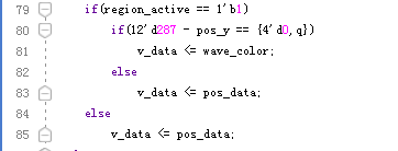
| Signal Name | Direction | Width (bit) | Description |
| pclk | in | 1 | Pixel clock |
| rst_n | in | 1 | Asynchronous reset, active low |
| wave_color | in | 24 | Waveform colour, rgb |
| adc_clk | in | 1 | adc module clock |
| adc_buf_wr | in | 1 | adc data write enable |
| adc_buf_addr | in | 12 | adc data write address |
| adc_buf_data | in | 8 | adc data, unsigned number |
| i_hs | in | 1 | Video horizontal sync input |
| i_vs | in | 1 | Video vertical sync input |
| i_de | in | 1 | Video data valid input |
| i_data | in | 24 | Video data input |
| o_hs | out | 1 | Video horizontal sync output with grid |
| o_vs | out | 1 | Video vertical sync output with grid |
| o_de | out | 1 | Video data valid output with grid |
| o_data | out | 24 | Video data output with grid |
Ports of the wav_display module
The RAM configuration is as follows:
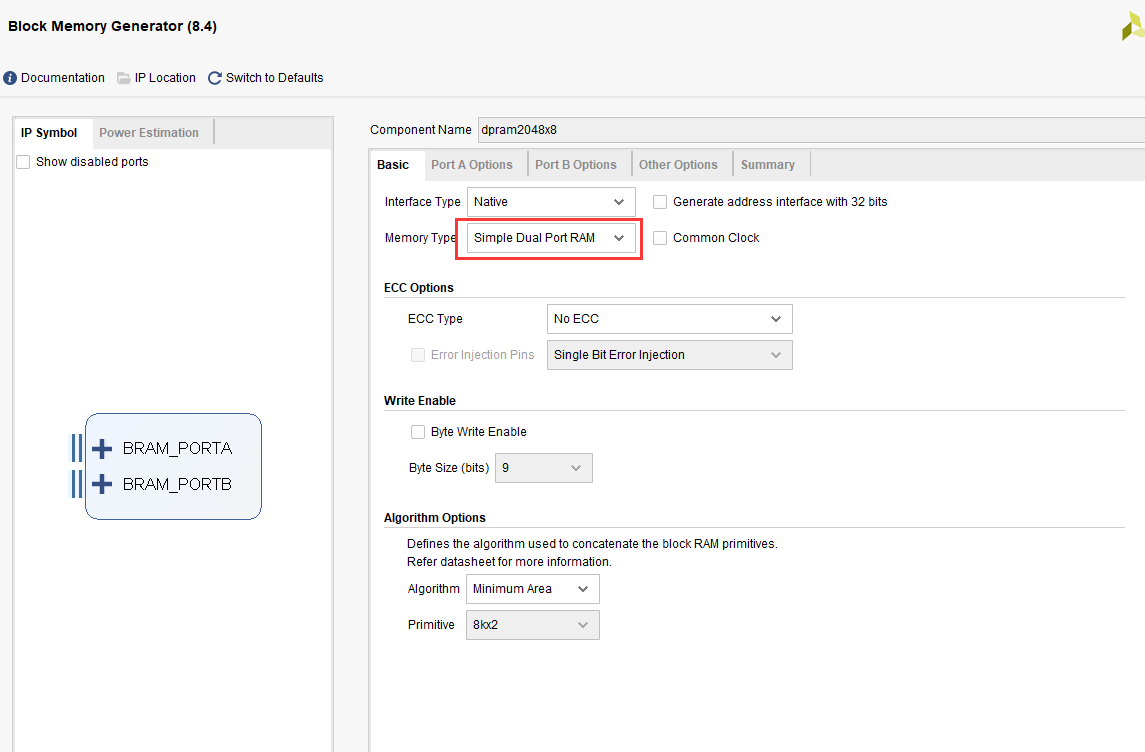
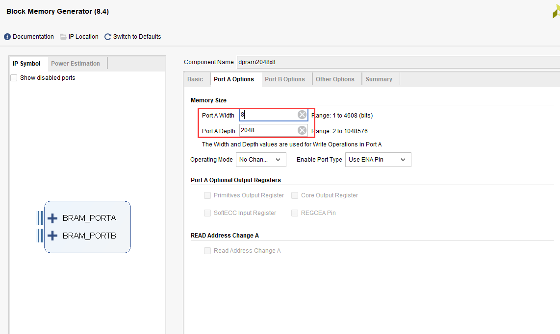
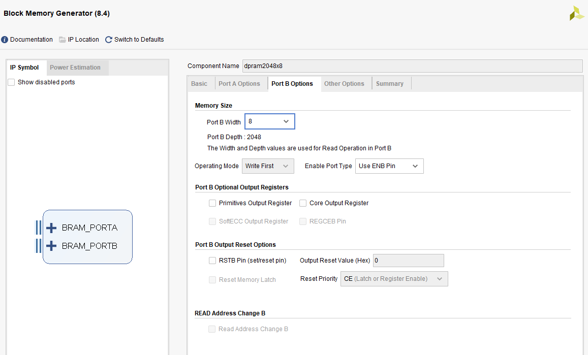
The timing_gen_xy module is a sub-module of the other modules and performs the coordinate generation of the video image: the x coordinate increases from left to right and the y coordinate increases from top to bottom.
| Signal Name | Direction | Width (bit) | Description |
| clk | in | 1 | System clock |
| rst_n | in | 1 | Asynchronous reset, active low |
| i_hs | in | 1 | Video horizontal sync input |
| i_vs | in | 1 | Video vertical sync input |
| i_de | in | 1 | Video data valid input |
| i_data | in | 24 | Video data input |
| o_hs | out | 1 | Video horizontal sync output |
| o_vs | out | 1 | Video vertical sync output |
| o_de | out | 1 | Video data valid output |
| o_data | out | 24 | Video data output |
| x | out | 12 | Coordinate x output |
| y | out | 12 | Coordinate y output |
Ports of the timing_gen_xy module
The xadc configuration is as follows
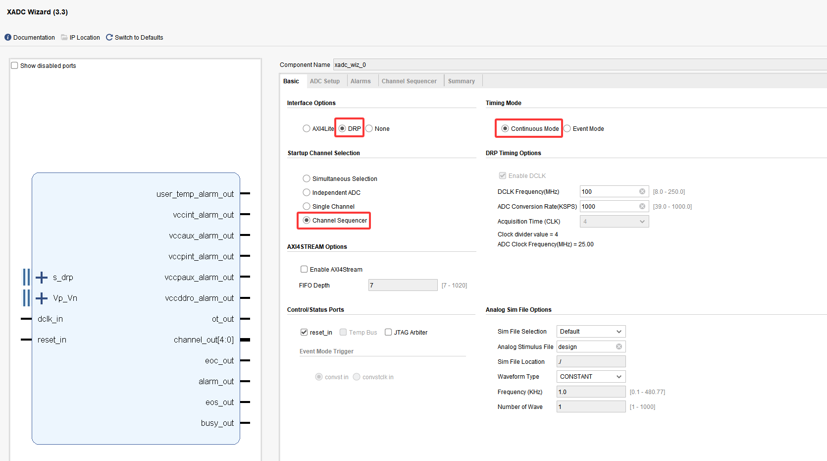
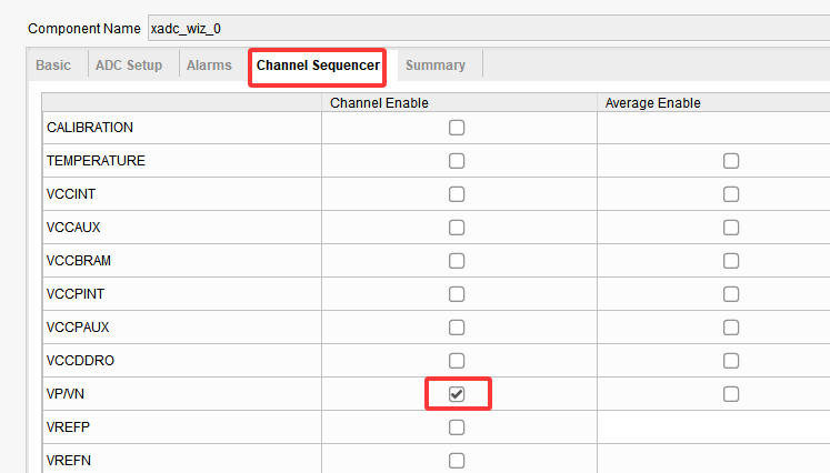
drp_master.v implements the read and write of the drp interface and connects to the DRP interface of the xadc.
drp_read_top.v implements the data read and write of the xadc and connects to drp_master.
According to document ug480, the status register of VPVN is 03h, so read_channel is configured as 3 when instantiating.
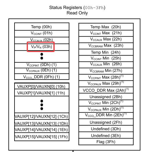
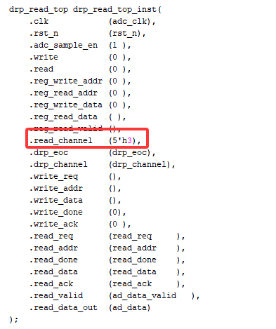
Also, the valid data is the upper 12 bits, so only the upper 12 bits are output.

12.3 Experiment Results
Connect the circuit as follows, connecting the SMA to the waveform generator. To make it convenient to observe the display effect, and for a better viewing result, set the waveform generator sampling frequency in the range 1KHz to 10KHz and the voltage amplitude to a maximum of 10V. Since only positive voltages can be acquired, a voltage offset must be set, for example an amplitude of 10V with an offset of 5V, or an amplitude of 5V with an offset of 2.5V. The result is the rendering at the very beginning of this chapter.
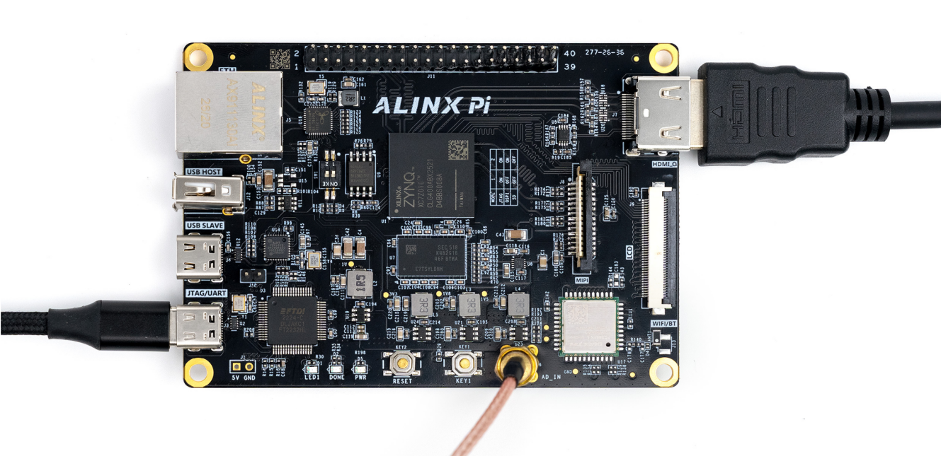
HDMI display hardware connection
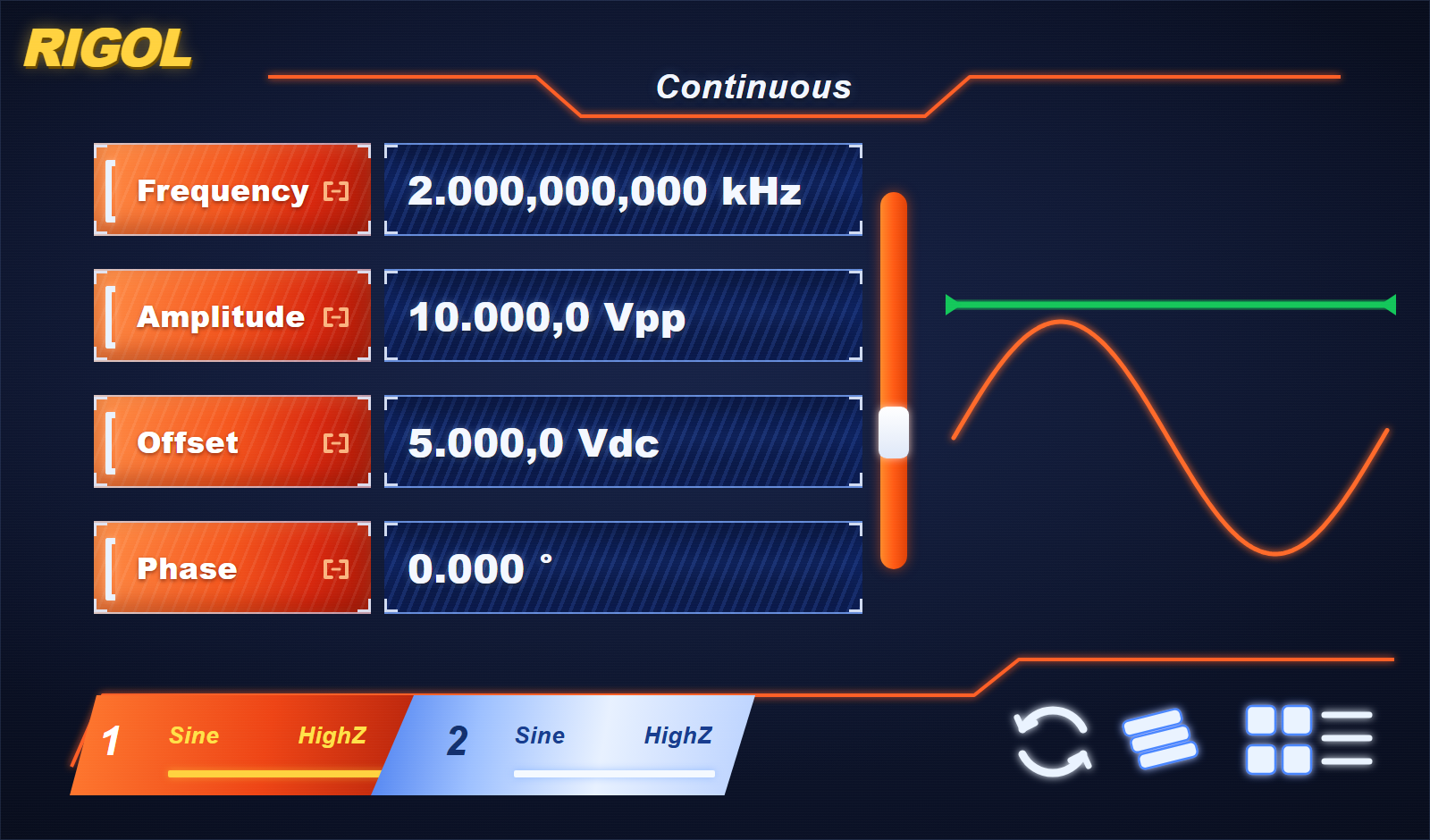
Waveform generator configuration
Waveform display result
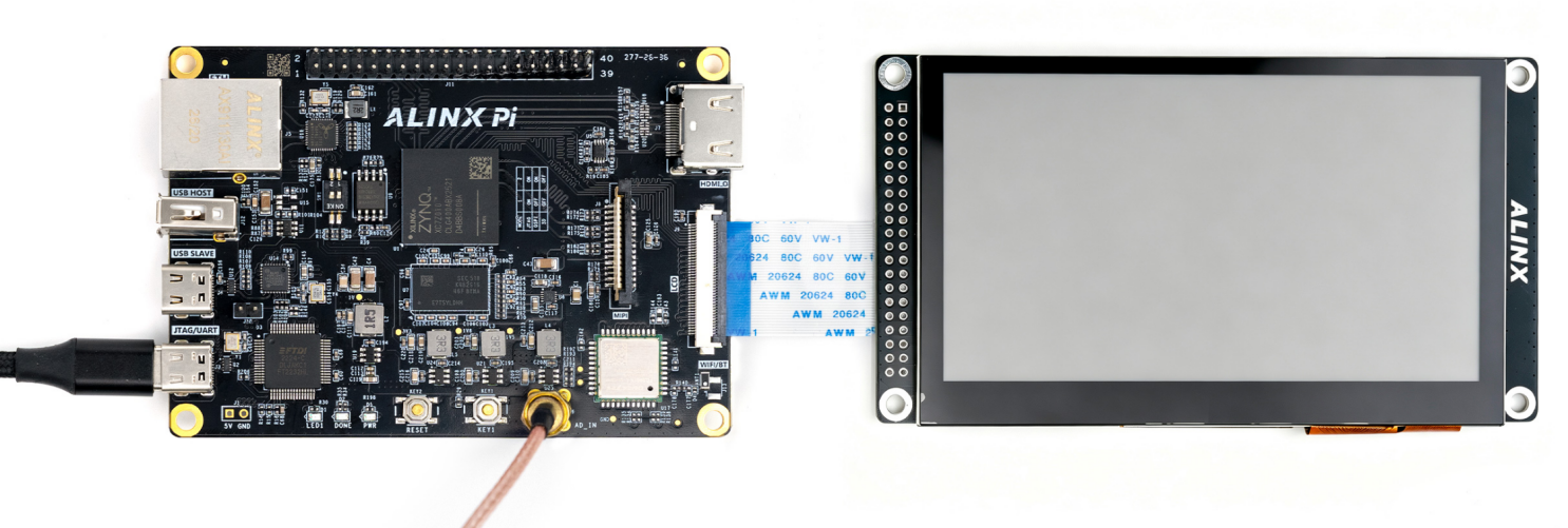
LCD panel connection
Appendix: Glossary of Terms
This appendix explains the abbreviations and technical terms used throughout this tutorial. Entries are listed alphabetically; the name in brackets is the full English form of an abbreviation, and the description gives the meaning and the role that the term plays in this tutorial.
A.1 List of Abbreviations
| Abbreviation | Full English Name | Description |
| ACP | Accelerator Coherency Port | A slave AXI port defined in the ARM multicore architecture that lets cacheless AXI masters in the PL, such as a DMA, access PS memory coherently. |
| ADC | Analog-to-Digital Converter | A circuit that converts an analog voltage into a digital code; the ZYNQ device contains the dual-channel 12-bit XADC. |
| AHB / APB | Advanced High-performance Bus / Advanced Peripheral Bus | Earlier AMBA buses with separate address and data phases that AXI replaced in ZYNQ designs. |
| AMBA | Advanced Microcontroller Bus Architecture | The ARM on-chip bus standard of which AXI is a part. |
| AXI | Advanced eXtensible Interface | A high-performance, high-bandwidth, low-latency on-chip bus protocol that defines how a master transfers data to and from a slave; every internal device in ZYNQ has an AXI interface. |
| AXI4 | Advanced eXtensible Interface 4 | The AXI generation included in AMBA 4.0; compared with AXI4-Lite it adds burst transfer, so a continuous block of addresses can be read or written in one transaction. |
| AXI4-Lite | AXI4 Lite | The lightweight AXI4 variant without burst transfer; each read or write accesses a single 32-bit word and it is used for low-speed peripherals and control registers. |
| AXI4-Stream | AXI4 Stream | An address-free AXI streaming interface that carries a continuous data flow from a source to a sink and is used for video, DSP and other real-time signal paths. |
| AXI-CDMA | AXI Central Direct Memory Access | A PL-side DMA engine that copies data from one memory location to another without involving the CPU. |
| AXI-Datamover | AXI DataMover | An IP core that converts AXI-HP to AXI4-Stream like AXI-DMA, but is controlled entirely by the PL while the PS remains passive. |
| AXI-DMA | AXI Direct Memory Access | An IP core that converts between the PS memory interface (AXI-HP) and an AXI4-Stream channel in the PL. |
| AXI-FIFO-MM2S | AXI FIFO Memory Map to Stream | An IP core that converts the general-purpose memory-mapped interface (AXI-GP) into an AXI4-Stream channel. |
| AXI-VDMA | AXI Video Direct Memory Access | A DMA IP core dedicated to two-dimensional data such as video frames and images. |
| BSP | Board Support Package | The drivers, libraries and configuration files that SDK generates for a specific hardware platform. |
| DDC | Display Data Channel | The HDMI/DVI signal line used to read the monitor EDID and to exchange HDCP keys. |
| DDR | Double Data Rate | The external synchronous DRAM attached to the PS memory controller; the PL reaches it through the AXI-HP ports. |
| DE | Data Enable | The video signal that marks the active pixel area of a line; pixels are valid only while DE is asserted. |
| DMA | Direct Memory Access | Data movement carried out by a dedicated controller instead of the CPU. |
| DRP | Dynamic Reconfiguration Port | The port through which the XADC registers are read and written while the design is running. |
| DVI | Digital Visual Interface | A digital display interface that uses the same TMDS signalling as HDMI. |
| EDID | Extended Display Identification Data | The data structure read over DDC that describes a monitor's supported resolutions and timings. |
| FIFO | First In, First Out | A memory that returns data in the order in which it was written; it has no address lines and is used for data buffering and clock-domain crossing. |
| FSBL | First Stage Boot Loader | The first program executed at power-up; it configures the PL and loads the next boot stage. |
| FSM | Finite State Machine | A circuit that steps through a defined set of states according to trigger conditions, implemented with always and case statements. |
| FWFT | First Word Fall Through | A FIFO read mode in which data is prefetched, so valid data is already on the output when rd_en is asserted. |
| GP | General Purpose (AXI-GP) | The four 32-bit general-purpose AXI ports of the PS (two master and two slave), each with a theoretical bandwidth of 600 MB/s. |
| GPIO | General-Purpose Input/Output | A software-configurable digital input or output pin. |
| HDCP | High-bandwidth Digital Content Protection | The content-protection scheme whose cipher keys are exchanged over the DDC line. |
| HDL | Hardware Description Language | A language such as Verilog or VHDL that describes digital hardware. |
| HDMI | High-Definition Multimedia Interface | A digital interface that carries high-definition video and audio as TMDS differential signals. |
| HP | High Performance (AXI-HP) | The four 64-bit high-bandwidth AXI ports through which the PL accesses PS memory (DDR and on-chip RAM) at up to 1200 MB/s. |
| I2C | Inter-Integrated Circuit | A two-wire serial bus on the PS side used for low-speed peripherals. |
| ILA | Integrated Logic Analyzer | Vivado's built-in online logic analyser; it captures internal signals at run time and stores them in on-chip block RAM. |
| IP | Intellectual Property (IP core) | A reusable logic block, supplied by Xilinx, by a third party or generated by the user, that is instantiated in a design. |
| JTAG | Joint Test Action Group | The debug and configuration interface used to program the device and to connect the ILA. |
| LCD | Liquid Crystal Display | The 4.3-inch 800x480 panel driven by the RGB output in Chapter 11. |
| LED | Light Emitting Diode | A diode used as an indicator; on this board the user LEDs are lit by a low level. |
| LVCMOS33 | Low-Voltage CMOS 3.3 V | The I/O standard assigned to pins located in a 3.3 V bank. |
| MIO | Multiplexed I/O | PS pins that can be mapped to functions such as UART, I2C, SD or GPIO; they are not constrained in the XDC file. |
| OCM | On-Chip Memory | The RAM inside the PS, also reachable from the PL through the AXI-HP ports. |
| OSD | On-Screen Display | The overlay of characters or graphics on top of the video image, used in Chapter 10 to show text over colour bars. |
| PL | Programmable Logic | The FPGA part of a ZYNQ device; it uses the same logic resources as the equivalent 7-series device. |
| PLL | Phase-Locked Loop | The clock generation block used to derive the pixel clock and its 5x serialisation clock from the 50 MHz board oscillator. |
| PS | Processing System | The ARM SoC part of a ZYNQ device; it contains the Cortex-A9 cores, memory controllers and peripherals and can run independently of the PL. |
| PWM | Pulse Width Modulation | A technique that varies the duty cycle of a square wave to control average power, used here to dim and brighten an LED. |
| RAM | Random Access Memory | Read/write memory; the block RAM inside the FPGA is used to build the RAM, ROM and FIFO experiments. |
| RGB | Red, Green, Blue | The 24-bit colour format with 8 bits per channel that is encoded into TMDS for the HDMI output. |
| ROM | Read-Only Memory | Memory whose contents are fixed at configuration time; in an SRAM-based FPGA it is built from block RAM preloaded with an initialisation file. |
| RTL | Register Transfer Level | The register-level view of a design; Vivado can draw an RTL schematic of the elaborated logic. |
| SDK | Software Development Kit | Xilinx's tool for writing and debugging ARM software against a Vivado hardware platform. |
| SMA | SubMiniature version A | The coaxial connector that brings the external analog signal to the XADC input. |
| SoC | System on Chip | A single chip that integrates a processor system, memory controllers, peripherals and programmable logic. |
| SRAM | Static Random Access Memory | The technology behind FPGA configuration memory, which is why a design is lost when the board is powered off. |
| TMDS | Transition Minimized Differential Signaling | The encoding and serialisation scheme used by HDMI and DVI: 8-bit data is encoded into 10 bits with minimised transitions and DC balance and then sent differentially. |
| UART | Universal Asynchronous Receiver/Transmitter | An asynchronous serial port on the PS side. |
| VGA | Video Graphics Array | The analog display standard whose line and frame timing is reused for the HDMI colour bar output. |
| XADC | Xilinx Analog-to-Digital Converter | The on-chip dual-channel 12-bit ADC with a 1 MSPS sampling rate, used in Chapter 12 to acquire and display waveforms. |
| XDC | Xilinx Design Constraints | The Tcl-based constraint file used by Vivado for pin, clock and group constraints. |
A.2 Technical Terms
| Term | Description |
| Active Video | The visible pixel area of a video line or frame, as opposed to the blanking interval. |
| Asynchronous Reset | A reset that takes effect immediately, independently of the clock, and whose signal must be listed in the sensitivity list. |
| AXI Interconnect | The interconnect matrix IP that connects one or more AXI masters to one or more AXI slaves; it supports up to 16 masters and 16 slaves in N-to-1, 1-to-N or N-to-M (crossbar and shared access) modes. |
| Behavioral Simulation | Simulation of the RTL source without synthesis, used here to check the design before a bitstream is generated. |
| Bitstream | The .bit configuration file produced by implementation and downloaded to the device over JTAG. |
| Blanking (Front Porch / Sync / Back Porch) | The non-display part of a video line, made up of the front porch, the sync pulse and the back porch; active video plus blanking makes up one line period. |
| Blocking Assignment | The = assignment in Verilog: statements execute in order and the value takes effect immediately; it is used in combinational logic and in assign statements. |
| Block Memory Generator | The Vivado IP that implements block RAM memories; its Memory Type option selects single-port RAM, simple dual-port RAM, true dual-port RAM or ROM. |
| BOOT.bin | The boot image built in SDK from the FSBL, the bitstream and u-boot.elf, which the PS reads from the SD card at power-up. |
| Character Dot Matrix | The bitmap of a character produced by the extraction tool and saved as a .coe file; one dot corresponds to one bit in ROM and to one pixel on screen. |
| Clocking Wizard | The Vivado IP used to configure a PLL or MMCM, here to generate the video pixel clock and its 5x serialisation clock. |
| COE File | A text initialisation file with the .coe extension that preloads ROM or RAM contents; the first line gives the radix, data lines end with a comma and the last line with a semicolon. |
| Colour Bar | A test pattern of eight vertical colour bars used to verify the HDMI and LCD output paths. |
| Combinational Logic | Logic whose output depends only on the present inputs and changes immediately when they change, without reference to a clock. |
| Continuous Assignment | The assign statement that drives a wire from an expression and models a combinational connection. |
| Cortex-A9 | The dual-core ARM application processor inside the PS, around which the ZYNQ device is built. |
| Custom IP | A user-defined IP core, normally generated with the Vivado wizard, that exposes AXI4-Lite, AXI4 or AXI4-Stream interfaces to the PS. |
| D Flip-flop | A one-bit register that captures its input on a clock edge; the basic building block of the sequential logic in Chapter 2. |
| Duty Cycle | The fraction of a PWM period during which the output is high, given by duty / 2^N x 100%. |
| Full Adder | An adder stage that also takes the carry from the lower bit into account. |
| Half Adder | An adder stage that adds two bits without an incoming carry and produces a sum and a carry. |
| Handshake (VALID / READY) | The AXI transfer mechanism: the master asserts VALID when its data is valid and the slave asserts READY when it can accept data; a transfer completes only when both are asserted. |
| Hardware Manager | The Vivado window used to connect over JTAG, detect the ARM and FPGA cores and program the device. |
| Implementation (Place and Route) | The step that maps the synthesised netlist onto device resources and routes the connections before a bitstream can be generated. |
| Instantiation | Placing an instance of a module inside another module and connecting its ports. |
| IP Catalog | The Vivado browser from which IP cores are searched for, configured and generated. |
| localparam | A constant visible only inside the module that cannot be overridden at instantiation; it is typically used for state names. |
| MARK_DEBUG | A synthesis attribute (MARK_DEBUG = true) that marks a signal so that Vivado can insert an ILA for it during Set Up Debug. |
| Mealy State Machine | A state machine whose outputs depend on both the current state and the inputs; implemented here in the one-segment style. |
| Memory-Mapped Access | Access in which a peripheral is mapped into an address space, so that reading and writing it is like reading and writing memory. |
| Memory Type | The Verilog declaration reg [n-1:0] mem[m-1:0], which defines m words of n bits and models RAM or ROM. |
| Moore State Machine | A state machine whose outputs depend only on the current state; implemented here in the three-segment style. |
| Multiplexer | A circuit that selects one of several inputs according to a select signal, as in the 4-to-1 multiplexer of Section 2.5.9. |
| Non-Blocking Assignment | The <= assignment: all right-hand sides are evaluated first and the results are updated at the end of the always block; used in sequential logic to avoid races. |
| One-segment / Three-segment Style | Coding styles for state machines: everything in a single always block, or separate always blocks for the state register, the next-state logic and the outputs. |
| Package | The package code in the part number, for example clg400 for the 400-pin package used on this development board. |
| Parameter | A constant that can be passed into a module at instantiation through #( ), which makes a design configurable and reusable. |
| Pin Constraint | The XDC properties PACKAGE_PIN and IOSTANDARD that bind a port to a physical pin and to a voltage standard. |
| Pixel Clock | The clock whose rate equals the pixel output rate; 74.25 MHz for 1280x720 at 60 Hz and 33 MHz for the 800x480 LCD panel. |
| Probe / Sample Data Depth | The ILA settings that define how many signals are captured and how many samples are stored per capture. |
| Race and Hazard | Ordering-dependent glitches in simulation that non-blocking assignment in sequential logic is used to avoid. |
| reg | The Verilog variable type that stores a value and must be assigned inside an always block. |
| Repository | A folder registered in Vivado through Add Repository that supplies third-party or user IP, such as the RGB to DVI encoder used in Chapter 9. |
| Sampling Rate | The number of conversions performed per second; the XADC converts at up to 1 MSPS. |
| Sensitivity List | The signal list in an always block that triggers re-evaluation; an asynchronous reset must be included in it while a synchronous signal must not. |
| Sequential Logic | Logic whose output depends on both the current inputs and the previous state of the circuit, clocked by a signal edge. |
| Set Up Debug | The Vivado wizard that inserts an ILA for the signals marked with MARK_DEBUG. |
| Shift Register | A chain of flip-flops that moves data one bit left or right on each clock edge. |
| Simple Dual-port RAM | A RAM with a write port and a separate read port, so that read and write operations can take place in the same cycle. |
| Single-port RAM | A RAM that shares one address port for both read and write. |
| Software-Hardware Co-Design | The ZYNQ development model in which ARM software, drivers and FPGA logic are designed and debugged together. |
| Speed Grade | The -1 or -2 suffix in the part number; a larger number means faster silicon, and faster grades are downward compatible with slower ones. |
| Synthesis | The step that turns RTL source into a gate-level netlist; it is also required before the timing constraint wizard can identify the clocks. |
| Testbench | A simulation-only module that instantiates the design under test and applies stimulus such as clocks, resets and data. |
| Timing Constraint | The XDC constraint that defines clock periods and I/O timing, for example create_clock -period 20 for a 50 MHz clock. |
| Tri-state Buffer | A driver that can be driven high, driven low or placed in high impedance (1'bz); it is used to build bidirectional I/O. |
| True Dual-port RAM | A RAM with two complete ports, each with its own address, data and control lines, so that two systems can access it independently. |
| Verilog Module | The basic design unit: a named block with a port list and a body of statements. |
| Voltage Divider | The resistor network on the board that scales a 0-10 V input down to the 0-1 V range accepted by the XADC. |
| wire | The Verilog net type that models a physical connection; it cannot store a value and is driven by assign. |
| 3-to-8 Decoder | A decoder that asserts one of eight outputs according to a 3-bit address. |
Contact information
Alinx Electronic Limited
Company Website: www.en.alinx.com
Service Hotline: +86 21 67676997
Technical Support:technical@alinx.com